

electrodynamics / Electromagnetic Field Theory - Bo Thide
.pdf6.1 CHARGED PARTICLES IN AN ELECTROMAGNETIC FIELD |
73 |
|
With the help of these, the radius four-vector x , considered as the generalised four-coordinate, and the invariant line element ds, defined in Equation (5.15) on page 56, we introduce the following eight partial differential equations:
@H(4) |
= |
|
dx |
|
(6.17a) |
|
@p |
|
ds |
||||
|
|
|
||||
@H(4) |
|
|
dp |
(6.17b) |
||
|
= |
|
|
|||
@x |
ds |
|||||
which form the four-dimensional Hamilton equations.
Our strategy now is to use Equation (6.15) on the facing page and Equations (6.17) above to derive an explicit algebraic expression for the canonically conjugate momentum four-vector. According to Equation (5.39) on page 61, a four-momentum has a zeroth (time) component which we can identify with the total energy. Hence we require that the component p0 of the conjugate fourmomentum vector defined according to Equation (6.15) on the preceding page be identical to the ordinary 3D Hamiltonian H and hence that this component solves the Hamilton equations Equations (6.14) on the facing page. This later consistency check is left as an exercise to the reader.
Using the definition of H(4), Equation (6.16) on the preceding page, and
the expression for L(4), Equation (6.3) on page 70, we obtain |
|
||
H(4) = p u L(4) = p u |
m0c2 |
u u qu A (x ) |
(6.18) |
2 |
|||
Furthermore, from the definition (6.15) of the conjugate four-momentum p , we see that
|
@L(4) |
@ |
|
m0c2 |
|
|
|||||
p = |
|
|
= |
|
|
|
u u +qu A (x ) |
||||
@u |
@u |
2 |
|||||||||
|
|
|
|
|
(6.19) |
||||||
= m0c2u +qA |
|
|
|||||||||
Inserting this into (6.18), we obtain |
|
||||||||||
H(4) = m0c2u u +qA u |
m0c2 |
u u qu A (x ) |
|||||||||
2 |
|||||||||||
|
|
m0c2 |
|
|
|
|
(6.20) |
||||
|
|
|
|
|
|
|
|||||
= |
|
|
u u |
|
|
|
|
|
|||
|
|
|
|
|
|
|
|||||
2 |
|
|
|
|
|
|
|
|
|||
Since the four-velocity scalar-multiplied by itself is u u = 1, we clearly see from Equation (6.20) above that H(4) is indeed a scalar invariant, whose value is simply
|
m0c2 |
||
H(4) = |
|
(6.21) |
|
2 |
|||
|
|
||
Draft version released 13th November 2000 at 22:01. |
Downloaded from http://www.plasma.uu.se/CED/Book |
|
|
74 |
INTERACTIONS OF FIELDS AND PARTICLES |
|
However, at the same time (6.19) provides the algebraic relationship
u = |
|
1 |
"p qA # |
(6.22) |
||||||||
m0c2 |
||||||||||||
and if this is used in (6.20) to eliminate u , one gets |
||||||||||||
|
|
|
m0c2 |
|
1 |
|
# 1 |
|
|
|||
H(4) = |
|
|
|
|
|
"p qA |
|
|
"p qA # |
|||
2 |
m0c2 |
|
m0c2 |
|||||||||
|
|
1 |
|
"p qA #"p qA # |
(6.23) |
|||||||
= |
|
|||||||||||
2m0c2 |
||||||||||||
|
|
1 |
|
"p p |
2qA p +q2A A # |
|||||||
= |
|
|||||||||||
2m0c2 |
||||||||||||
That this four-Hamiltonian yields the correct covariant equation of motion can be seen by inserting it into the four-dimensional Hamilton's equations (6.17) and using the relation (6.22):
@H(4) |
|
q |
|
|
|
@A |
|||
|
= |
|
(p qA ) |
|
|
|
|||
@x |
m0c2 |
@x |
|||||||
|
|
q |
2 |
|
@A |
||||
|
= |
|
m0c |
u |
|
|
|
||
|
m0c2 |
|
@x |
||||||
|
|
|
|
|
(6.24) |
||||
=qu @A
@x
=dp = moc2 du q @A u ds ds @x
where in the last step Equation (6.19) on the preceding page was used. Rearranging terms, and using Equation (5.77) on page 67, we obtain
|
2 du |
|
@A |
|
@A |
|
|
(6.25) |
|||
m0c |
|
|
= qu |
|
|
|
|
|
= qu |
F |
|
|
ds |
|
@x |
@x |
|||||||
which is identical to the covariant equation of motion Equation (6.13) on page 72. We can then safely conclude that the Hamiltonian in question is correct.
Using the fact that expression (6.23) above for H(4) is equal to the scalar value m0c2=2, as derived in Equation (6.21) on the preceding page, the fact that
p = (p0;cp) |
(6.26a) |
A = ( ;cA) |
(6.26b) |
p p = (p0)2 c2(p)2 |
(6.26c) |
A p = p0 c2(p A) |
(6.26d) |
A A = 2 c2(A)2 |
(6.26e) |
Downloaded from http://www.plasma.uu.se/CED/Book |
Draft version released 13th November 2000 at 22:01. |
|
|
6.1 CHARGED PARTICLES IN AN ELECTROMAGNETIC FIELD |
75 |
|
and Equation (6.19) on page 73, we obtain the equation |
|
|
||||
m0c2 |
1 |
(p0)2 c2(p)2 2q p0 +2qc2(p A) +q2 2 q2c2 |
(A)2 |
|
||
|
|
= |
|
|
||
2 |
2m0c2 |
|
||||
|
|
|
|
|
(6.27) |
|
which is a second order algebraic equation in p0 which can be written |
|
|
||||
(m0c2)2 = (p0)2 2q p0 c2(p)2 +2qc2(p A) q2c2(A)2 +q2 2 |
(6.28) |
|||||
or |
|
|
|
|
|
|
(p0)2 2q p0 c2 (p)2 2qp A +q2(A)2 +q2 2 m20c4
(6.29)
= (p0)2 2q p0 c2(p qA)2 +q2 2 m20c4 = 0
with two possible solutions
p0 = q c? (p qA)2 +m02c2 |
(6.30) |
Since the fourth component (time component) p0 of the four-momentum p is the total energy, the positive solution in (6.30) must be identified with the ordinary Hamilton function H. This means that
H p0 = q +c? (p qA)2 +m02c2 |
(6.31) |
is the ordinary 3D Hamilton function for a charged particle moving in scalar and vector potentials associated with prescribed electric and magnetic fields.
The ordinary Lagrange and Hamilton functions L and H are related to each other by the 3D transformation [cf. the 4D transformation (6.16) between L(4) and H(4)]
L = p v H |
(6.32) |
Using the explicit expressions (Equation (6.31)) and (Equation (6.32) above), we obtain the explicit expression for the ordinary 3D Lagrange function
L =p v q c? (p qA)2 +m02c2 |
(6.33) |
|||||
and if we make the identification |
|
|||||
|
?m0v |
|
||||
p qA = |
|
|
|
|
= mv |
(6.34) |
|
|
|
|
|||
|
1 |
v2 |
|
|||
|
c2 |
|
|
|||
Draft version released 13th November 2000 at 22:01. |
Downloaded from http://www.plasma.uu.se/CED/Book |
|
|
76 |
INTERACTIONS OF FIELDS AND PARTICLES |
|
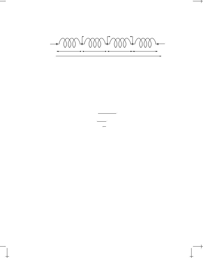
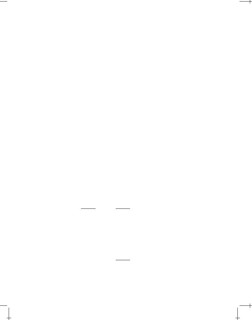
|
i 1 |
i |
i+1 |
|
m |
m |
m |
m |
m |
k |
k |
k |
k |
|
a |
a |
a |
a |
x |
FIGURE 6.1: A one-dimensional chain consisting of N discrete, identical mass points m, connected to their neighbours with identical, ideal springs with spring constants k. The equilibrium distance between the neighbouring mass points is a and i 1(t), i(t), i+1(t) are the instantaneous deviations, along the x axis, of positions of the (i 1)th, ith, and (i +1)th
mass point, respectively.
where the quantity mv is called the kinetic momentum, we can rewrite this expression for the ordinary Lagrangian as follows:
L = qA v +mv2 q c? m2v2 m20c2
(6.35)
= q +qA v m0c2 1 v2 c2
What we have obtained is the correct expression for the Lagrangian describing the motion of a charged particle in scalar and vector potentials associated with prescribed electric and magnetic fields.
6.2 Covariant Field Theory
So far, we have considered two classes of problems. Either we have calculated the fields from given, prescribed distributions of charges and currents, or we have derived the equations of motion for charged particles in given, prescribed fields. Let us now put the fields and the particles on an equal footing and present a theoretical description which treats the fields, the particles, and their interactions in a unified way. This involves transition to a field picture with an infinite number of degrees of freedom. We shall first consider a simple mechanical problem whose solution is well known. Then, drawing inferences from this model problem, we apply a similar view on the electromagnetic problem.
Downloaded from http://www.plasma.uu.se/CED/Book |
Draft version released 13th November 2000 at 22:01. |
|
|
6.2 COVARIANT FIELD THEORY |
77 |
|
6.2.1 Lagrange-Hamilton formalism for fields and interactions
Consider N identical mass points, each with mass m and connected to its neighbour along a one-dimensional straight line, which we choose to be the x axis, by identical ideal springs with spring constants k. At equilibrium the mass points are at rest, distributed evenly with a distance a to their two nearest neighbours. After perturbation, the motion of mass point i will be a one-dimensional oscillatory motion along xˆ. Let us denote the magnitude of the deviation for mass point i from its equilibrium position by i(t)xˆ.
The solution to this mechanical problem can be obtained if we can find a Lagrangian (Lagrange function) L which satisfies the variational equation
L( i;˙i;t)dt = 0 |
(6.36) |
According to Equation (M.84) on page 176, the Lagrangian is L = T V where T denotes the kinetic energy and V the potential energy of a classical mechanical system with conservative forces. In our case the Lagrangian is
|
1 |
N |
|
|
L = |
å m˙i2 k( i+1 i)2 |
(6.37) |
||
2 |
||||
|
|
i=1 |
|
Let us write the Lagrangian, as given by Equation (6.37), in the following way:
|
|
N |
|
|
|
|
|
|
|
|
|
|
|
L = åa@ i |
|
|
|
|
|
|
(6.38) |
||||||
|
|
i=1 |
|
|
|
|
|
|
|
|
|
|
|
Here, |
|
|
|
|
|
|
|
|
|
|
|
|
|
@ |
i |
= |
1 |
|
m |
˙ |
2 |
|
ka |
i+1 i |
2 |
|
(6.39) |
|
|
i |
|
||||||||||
|
2 |
a |
|
a |
|
|
|
||||||
is the so called linear Lagrange density. If we now let N !1 and, at the same time, let the springs become infinitesimally short according to the following scheme:
|
a ! dx |
|
|
(6.40a) |
|||
|
m |
! |
dm |
= |
linear mass density |
(6.40b) |
|
|
a |
dx |
|||||
ka ! Y |
|
Young's modulus |
(6.40c) |
||||
i+1 i |
|
@ |
|
|
|
(6.40d) |
|
a |
! @x |
|
|
||||
|
|
|
|||||
Draft version released 13th November 2000 at 22:01. |
Downloaded from http://www.plasma.uu.se/CED/Book |
|
|

78 |
INTERACTIONS OF FIELDS AND PARTICLES |
|
we obtain |
|
|
|
|
|
|
|
|
|
|
|
|
|
L = @ dx |
|
|
|
|
|
|
|
|
(6.41) |
||||
where |
|
|
|
|
|
|
|
|
|
|
|
|
|
|
|
@ @ |
|
1 |
@ 2 |
|
@ |
2; |
|||||
@ |
; |
|
; |
|
;t = |
|
: |
|
|
Y |
|
|
(6.42) |
@t |
@x |
2 |
@t |
@x |
|||||||||
Notice how we made a transition from a discrete description, in which the mass points were identified by a discrete integer variable i =1;2;:::;N, to a continuous description, where the infinitesimal mass points were instead identified by a continuous real parameter x, namely their position along xˆ.
A consequence of this transition is that the number of degrees of freedom for the system went from the finite number N to infinity! Another consequence is that @ has now become dependent also on the partial derivative with respect to x of the “field coordinate” . But, as we shall see, the transition is well worth the price because it allows us to treat all fields, be it classical scalar or vectorial fields, or wave functions, spinors and other fields that appear in quantum physics, on an equal footing.
Under the assumption of time independence and fixed endpoints, the variation principle (6.36) on the previous page yields:
where the variation is arbitrary (and the endpoints fixed). This means that the integrand itself must vanish. If we introduce the functional derivative
Ldt |
|
|
|
|
|
|
|
|
|
|
|
|
|
|
|
|
|
|
|
|
|
|
|
|
|
|
||
= A @ ; |
@ |
; |
|
@ |
|
dx dt |
|
|
|
|
|
|
|
|
|
|||||||||||||
|
|
|
|
|
|
|
|
|
|
|
|
|||||||||||||||||
|
|
|
|
|
|
|
@t |
@x |
|
|
|
|
|
|
|
|
|
|
|
|
|
|
(6.43) |
|||||
|
|
|
|
|
|
|
|
|
|
|
|
|
|
|
|
|
|
|
|
|
|
|
|
|
|
|
|
|
|
|
|
@@ |
|
|
|
|
|
@@ |
|
|
@ |
|
|
@@ |
|
@ |
|
||||||||||
= A CBD |
|
+ |
|
|
|
|
|
|
|
|
+ |
|
|
|
|
|
|
dx dt |
|
|||||||||
|
|
|
@ |
@t |
|
@ |
@x |
|
||||||||||||||||||||
|
|
|
|
|
|
|
|
@ t |
@ x |
|
|
|
|
|||||||||||||||
= 0 |
|
|
|
|
|
|
|
|
|
|
|
|
|
|
|
|
|
|
|
|
|
|
|
|
|
|
|
|
The last integral can be integrated by parts. This results in the expression |
||||||||||||||||||||||||||||
|
@@ |
|
@ |
@@ |
|
|
@ |
|
|
|
@@ |
|
68 EF dx dt = 0 |
(6.44) |
||||||||||||||
|
|
|
|
|
|
|
|
|
|
35 |
|
|||||||||||||||||
A DCB |
@t |
35@ @t 86 |
@x |
@ @x |
||||||||||||||||||||||||
|
|
|
|
|
|
|
|
|
|
|
|
|
|
|
|
|
|
|
|
|
|
|
|
|
|
|||
@ |
@@ |
|
@ @@ |
|
(6.45) |
||
|
= |
|
|
|
|
||
|
@x 35@ @x 68 |
||||||
Downloaded from http://www.plasma.uu.se/CED/Book |
Draft version released 13th November 2000 at 22:01. |
|
|
6.2 COVARIANT FIELD THEORY |
79 |
|
we can express this as
@ |
|
@ |
@@ |
|
= 0 |
(6.46) |
|
|
|
|
|
|
|||
|
@t |
35@ @t 86 |
|||||
which is the one-dimensional Euler-Lagrange equation.
Inserting the linear mass point chain Lagrangian density, Equation (6.42) on the facing page, into Equation (6.46) above, we obtain the equation of motion for our one-dimensional linear mechanical structure. It is:
|
@2 |
Y |
@2 |
|
@2 |
@2 |
= 0 |
(6.47) |
|||
|
|
|
= |
|
|
|
|
|
|||
@t2 |
@x2 |
Y |
@t2 |
@x2 |
|||||||
i.e., the one-dimensional wave equation for compression waves which propag- p
ate with phase speed v = Y= along the linear structure.
A generalisation of the above 1D results to a three-dimensional continuum is straightforward. For this 3D case we get the variational principle
Ldt = @ d3xdt
=G @ ; @ d4x
@x
(6.48)
|
@@ |
|
@ |
@@ |
|
|
d4x |
||
= A BD |
|
|
|
|
|
|
|||
@x 53@ |
@ |
86 FE |
|||||||
|
|
x |
|
||||||
= 0 |
|
|
|
|
|
|
|
|
|
where the variation is arbitrary and the endpoints are fixed. This means that the integrand itself must vanish:
@@ |
@ |
@@ |
|
|
= 0 |
(6.49) |
|||
|
|
|
|
|
|
|
|
||
|
@x |
35@ |
@ |
86 |
|||||
|
x |
|
|
||||||
This constitutes the three-dimensional Euler-Lagrange equations.
Introducing the three-dimensional functional derivative
@ |
@@ |
|
@ |
@@ |
|
(6.50) |
||
|
= |
|
|
|
|
|
||
|
|
@xi |
53@ @xi 86 |
|||||
Draft version released 13th November 2000 at 22:01. |
Downloaded from http://www.plasma.uu.se/CED/Book |
|
|
80 |
INTERACTIONS OF FIELDS AND PARTICLES |
|
we can express this as
@ |
|
@ |
@@ |
|
= 0 |
(6.51) |
|
|
|
|
|
|
|||
|
@t |
35@ @t 86 |
|||||
I analogy with particle mechanics (finite number of degrees of freedom), we may introduce the canonically conjugate momentum density
(x ) = (t;x) = |
@@ |
|
|
|
|
|
|
|
(6.52) |
|||
@ @t |
|
|
|
|
|
|||||||
|
|
|
|
|
|
|
|
|
||||
and define the Hamilton density |
|
|
|
|
|
|||||||
|
@ |
|
@ |
|
@ |
|
@ |
|
||||
H ; ; |
|
; t = |
|
|
@ ; |
|
; |
|
|
(6.53) |
||
@xi |
@t |
@t |
@xi |
|||||||||
If, as usual, we differentiate this expression and identify terms, we obtain the following Hamilton density equations
@ |
= |
@ |
|
(6.54a) |
||
@ |
@t |
|||||
|
|
|||||
H |
= |
@ |
(6.54b) |
|||
|
|
|||||
|
@t |
|||||
The Hamilton density functions are in many ways similar to the ordinary
Hamilton functions and lead to similar results.
The electromagnetic field
Above, when we described the mechanical field, we used a scalar field (t;x). If@ we want to describe the electromagnetic field in terms of a Lagrange density and Euler-Lagrange equations, it comes natural to express @ in terms of
the four-potential A (x ).
The entire system of particles and fields consists of a mechanical part, a field part and an interaction part. We therefore assume that the total Lagrange density @ tot for this system can be expressed as
@ tot = @ mech +@ inter +@ field |
(6.55) |
where the mechanical part has to do with the particle motion (kinetic energy). It is given by L(4)=V where L(4) is given by Equation (6.2) on page 70 and V is
Downloaded from http://www.plasma.uu.se/CED/Book |
Draft version released 13th November 2000 at 22:01. |
|
|
6.2 COVARIANT FIELD THEORY |
81 |
|
the volume. Expressed in the rest mass density 0m, the mechanical Lagrange density can be written
@ mech = |
1 |
0 c2u u |
(6.56) |
|
|||
2 |
m |
|
|
The @ inter part which describes the interaction between the charged particles and the external electromagnetic field. A convenient expression for this interaction Lagrange density is
@ inter = j A |
(6.57) |
For the field part @ field we choose the difference between magnetic and electric energy density (in analogy with the difference between kinetic and potential energy in a mechanical field). Using the field tensor, we express this
field Lagrange density as
@ field = |
1 |
"0F F |
|
(6.58) |
||||
4 |
|
|||||||
|
|
|
|
|
|
|
|
|
so that the total Lagrangian density can be written |
|
|||||||
@ tot = |
1 |
|
0 |
c2u u + j A + |
1 |
"0F F |
(6.59) |
|
|
|
|||||||
2 |
|
|
m |
4 |
|
|
||
From this we can calculate all physical quantities.
FIELD ENERGY DIFFERENCE EXPRESSED IN THE FIELD TENSOR
Show, by explicit calculation, that |
|
|
|
|
|
|
|||
F F = 2(c2 B2 E2) |
|
|
|
|
|
|
(6.60) |
||
From formula (5.77) on page 67 we recall that |
|
|
|
|
|||||
|
|
0 |
Ex |
Ey |
Ez |
|
|||
F =@ A |
|
@ A = KJIEx |
0 |
cBz |
cBy |
(6.61) |
|||
|
Ey |
cBz |
0 |
|
cBx |
|
|||
|
|
|
|||||||
|
|
Ez cBy |
cBx |
|
0 OLNM |
||||
and from formula (5.76) on page 66 that |
|
|
|
|
|
||||
|
|
0 |
Ex |
Ey |
|
Ez |
|
||
F = @ A |
|
@ A = IJK Ex |
0 |
cBz |
|
cBy |
(6.62) |
||
|
|
Ey |
cBz |
0 |
|
cBx |
|
||
|
|
|
|
|
|||||
|
|
Ez |
cBy |
cBx |
|
|
0 |
OLNM |
|
where denotes the row number and the column number. Then, Einstein summation
EXAMPLE
6.1
Draft version released 13th November 2000 at 22:01. |
Downloaded from http://www.plasma.uu.se/CED/Book |
|
|
82 |
|
|
|
|
|
|
|
INTERACTIONS OF FIELDS AND PARTICLES |
|
||||||||
|
and direct substitution yields |
|
|
|
|
|
|
||||||||||
|
|
F F = F00F00 +F01F01 +F02F02 +F03F03 |
|
|
|
||||||||||||
|
|
|
+F10F10 +F11F11 +F12F12 +F13F13 |
|
|
|
|||||||||||
|
|
|
+F20F20 +F21F21 +F22F22 +F23F23 |
|
|
|
|||||||||||
|
|
|
+F30F30 +F31F31 +F32F32 +F33F33 |
|
|
|
|||||||||||
|
|
|
=0 E2x Ey2 Ez2 |
|
|
|
(6.63) |
|
|
||||||||
|
|
|
E2x +0 +c2 Bz2 +c2 By2 |
|
|
|
|
|
|
||||||||
|
|
|
Ey2 +c2 Bz2 +0 +c2 B2x |
|
|
|
|
|
|
||||||||
|
|
|
Ez2 +c2 By2 +c2 B2x +0 |
|
|
|
|
|
|
||||||||
|
|
|
= 2E2x 2Ey2 2Ez2 +c2 B2x +c2 By2 +c2 Bz2 |
|
|
|
|||||||||||
|
|
|
= 2E2 +2c2 B2 = 2(c2 B2 E2) |
QED |
|
||||||||||||
|
|
|
|
|
|
|
|
|
|
|
|
|
|
|
|
||
|
|
|
|
|
|
|
|
|
|
|
|
|
|
END OF EXAMPLE 6.1 |
|
||
|
|
|
|
|
|
|
|
|
|
|
|
|
|
|
|||
|
Using @ tot in the 3D Euler-Lagrange equations, Equation (6.49) on page 79 |
|
|||||||||||||||
|
(with replaced by A ), we can derive the dynamics for the whole system. For |
|
|||||||||||||||
|
instance, the electromagnetic part of the Lagrangian density |
|
|
|
|||||||||||||
|
@ EM = @ inter +@ field = j A + |
1 |
"0F F |
(6.64) |
|
|
|||||||||||
|
4 |
|
|
||||||||||||||
|
|
|
|
|
|
|
|
|
|
|
|
|
|
|
|
|
|
|
inserted into the Euler-Lagrange equations, expression (6.49) on page 79, yields |
|
|||||||||||||||
|
two of Maxwell's equations. To see this, we note from Equation (6.64) above |
|
|||||||||||||||
|
and the results in Example 6.1 that |
|
|
|
|
|
|
||||||||||
|
|
@@ EM |
= j |
|
|
|
|
|
|
|
|
|
|
|
(6.65) |
|
|
|
|
A |
|
|
|
|
|
|
|
|
|
|
|
|
|
||
|
|
|
|
|
|
|
|
|
|
|
|
|
|
|
|
|
|
|
Furthermore, |
|
|
|
|
|
|
|
|
|
|
|
|
|
|
|
|
|
|
@@ EM |
"0 |
@ |
|
|
|
F F # |
|
|
|
||||||
|
|
@ |
= |
|
|
@ |
|
|
|
|
|
|
|||||
|
|
|
|
|
|
|
|||||||||||
|
|
@( A ) 4 |
@(@ A ) " |
|
|
|
|||||||||||
|
|
|
|
"0 |
@ |
|
|
(@ A @ A )(@ A @ A ) |
|
|
|
||||||
|
|
|
= |
|
|
@ |
|
|
|
|
|
||||||
|
|
|
4 |
@(@ A ) |
|
|
|
||||||||||
|
|
|
|
"0 |
@ |
|
@ A @ A @ A @ A |
(6.66) |
|
|
|||||||
|
|
|
= |
|
|
@ |
|
|
|
||||||||
|
|
|
4 |
@(@ A ) |
|
|
|||||||||||
|
|
|
|
|
|
|
|
|
|
|
|
|
@ A @ A +@ A @ A |
|
|
|
|
|
|
|
|
"0 |
@ |
"@ A @ A @ A @ A # |
|
|
|
||||||||
|
|
|
= |
|
|
@ @(@ A ) |
|
|
|
||||||||
|
|
|
2 |
|
|
|
|||||||||||
Downloaded from http://www.plasma.uu.se/CED/Book |
Draft version released 13th November 2000 at 22:01. |
|
|