electrodynamics / Electromagnetic Field Theory - Bo Thide

the expression

inserting this expression and d = 2 sin d into formula (8.9) on page 100 and integrating over , we find that the total radiated power from the antenna is

is called the radiation resistance. For the technologically important case of a half-wave antenna, i.e., for L ==2 or kL = , formula (8.18) above reduces to

The integral in (8.21) can be evaluated numerically. It can also be evaluated

1:22

where in the last step the Euler-Mascheroni constant = 0:5772 ::: and the cosine integral Ci(x) were introduced. Inserting this into the expression Equation (8.21) on the preceding page we obtain the value Rrad(=2) 73 .

8.4 Multipole radiation

In the general case, and when we are interested in evaluating the radiation far from the source volume, we can introduce an approximation which leads to a multipole expansion where individual terms can be evaluated analytically. We shall use Hertz' method to obtain this expansion.

8.4.1 The Hertz potential

Let us consider the continuity equation, which, according to expression (1.21) on page 9, can be written

and compare with Equation (8.23) on the facing page, we see that (t;x) satisfies this continuity equation. Furthermore, if we compare with the electric polarisation [cf. Equation (7.9) on page 89], we see that the quantity is related to the “true” charges in the same way as P is related to polarised charge. Therefore, is referred to as the polarisation vector.

We introduce a further potential e with the following property

where and A are the electromagnetic scalar and vector potentials, respectively. As we see, e acts as a “super-potential” in the sense that it is a potential from which we can obtain other potentials. It is called the Hertz' vector or polarisation potential and, as can be seen from (8.24) and (8.25), it satisfies the inhomogeneous wave equation

This equation is of the same type as Equation (3.19) on page 38, and has therefore the retarded solution

with Fourier components

we see that we can calculate the magnetic and electric fields, respectively, as follows

Clearly, the last equation is valid only outside the source volume, where r E = 0. Since we are mainly interested in the fields in the far zone, a long distance from the source region, this is no essential limitation.

Assume that the source region is a limited volume around some central point x0 far away from the field (observation) point x. Under these assumptions, we can expand expression (8.27) on the previous page the Hertz' vector,

due to the presence of non-vanishing (tret0 ;x0) in the vicinity of x0, in a formal series. For this purpose we recall from potential theory that

n=0

where

eikjx x0j

jx x0j is a Green´s function

is the angle between x0 x0 and x x0

Pn(cos ) is the Legendre polynomial of order n

jn(k x0 x0 ) is the spherical Bessel function of the first kind of order n h(1)n (k jx x0j) is the spherical Hankel function of the first kind of order n

According to the addition theorem for Legendre polynomials, we can write

where Pmn is an associated Legendre polynomial and, in spherical polar coordinates,

Inserting Equation (8.31), together with Equation (8.32) above, into Equation (8.28) on the preceding page, we can in a formally exact way expand the Fourier component of the Hertz' vector as

!(x0) jn(k x0 x0 ) Pn m(cos 0) e im'0 d3x0

V

We notice that there is no dependence on x x0 inside the integral; the integrand is only dependent on the relative source vector x0 x0.

We are interested in the case where the field point is many wavelengths away from the well-localised sources, i.e., when the following inequalities

hold. Then we may to a good approximation replace h(1)n with the first term in its asymptotic expansion:

and replace jn with the first term in its power series expansion:

Inserting these expansions into Equation (8.34) on the preceding page, we obtain the multipole expansion of the Fourier component of the Hertz' vector

This expression is approximately correct only if certain care is exercised; if many e!(n) terms are needed for an accurate result, the expansions of the spherical Hankel and Bessel functions used above may not be consistent and must be replaced by more accurate expressions. Taking the inverse Fourier transform of e! will yield the Hertz' vector in time domain, which inserted into Equation (8.29) on page 105 will yield C. The resulting expression can then in turn be inserted into Equation (8.30) on page 105 in order to obtain the radiation fields.

For a linear source distribution along the polar axis, = in expression (8.38b), and Pn(cos ) gives the angular distribution of the radiation. In the general case, however, the angular distribution must be computed with the help of formula (8.32) on the preceding page. Let us now study the lowest order contributions to the expansion of Hertz' vector.

8.4.2 Electric dipole radiation

where p! = V !(x0)d3x0 is the Fourier component of the electric dipole moment; cf. Equation (7.2) on page 87 which describes the static dipole moment.

If a spherical coordinate system is chosen with its polar axis along p!, the components of e!(0) are

Evaluating formula (8.29) on page 105 for the help vector C, with the spherically polar components (8.40) of e(0)! inserted, we obtain

Applying this to Equation (8.30) on page 105, we obtain directly the Fourier components of the fields

Keeping only those parts of the fields which dominate at large distances (the radiation fields) and recalling that the wave vector k = k(x x0)=jx x0j where k =!=c, we can now write down the Fourier components of the radiation parts of the magnetic and electric fields from the dipole:

These fields constitute the electric dipole radiation, also known as E1 radiation.

8.4.3 Magnetic dipole radiation

The next term in the expression (8.38b) on page 107 for the expansion of the Fourier transform of the Hertz' vector is for n = 1:

i.e., as the sum of two parts, the first being symmetric and the second antisymmetric in the indices i; j. We note that the antisymmetric part can be written as

Hence, we can write the antisymmetric part of the integral in formula (8.44) on the preceding page as

1(x x0) !(x0) (x0 x0) dV0

2V

where we introduced the Fourier transform of the magnetic dipole moment

The final result is that the antisymmetric, magnetic dipole, part of e!(1) can be written

In analogy with the electric dipole case, we insert this expression into Equation (8.29) on page 105 to evaluate C, with which Equations (8.30) on page 105 then gives the B and E fields. Discarding, as before, all terms belonging to the near fields and transition fields and keeping only the terms that dominate at large distances, we obtain

which are the fields of the magnetic dipole radiation (M1 radiation).

8.4.4 Electric quadrupole radiation

The symmetric part e!;sym(1) of the n = 1 contribution in the Equation (8.38b) on page 107 for the expansion of the Hertz' vector can be expressed in terms

of the electric quadrupole tensor, which is defined in accordance with Equation (7.3) on page 87:

Again we use this expression in Equation (8.29) on page 105 to calculate the fields via Equations (8.30) on page 105. Tedious, but fairly straightforward algebra (which we will not present here), yields the resulting fields. The radiation components of the fields in the far field zone (wave zone) are given by

This type of radiation is called electric quadrupole radiation or E2 radiation.

8.5 Radiation from a localised charge in arbitrary motion

The derivation of the radiation fields for the case of the source moving relative to the observer is considerably more complicated than the stationary cases studied above. In order to handle this non-stationary situation, we use the retarded potentials (3.36) on page 41 in Chapter 3

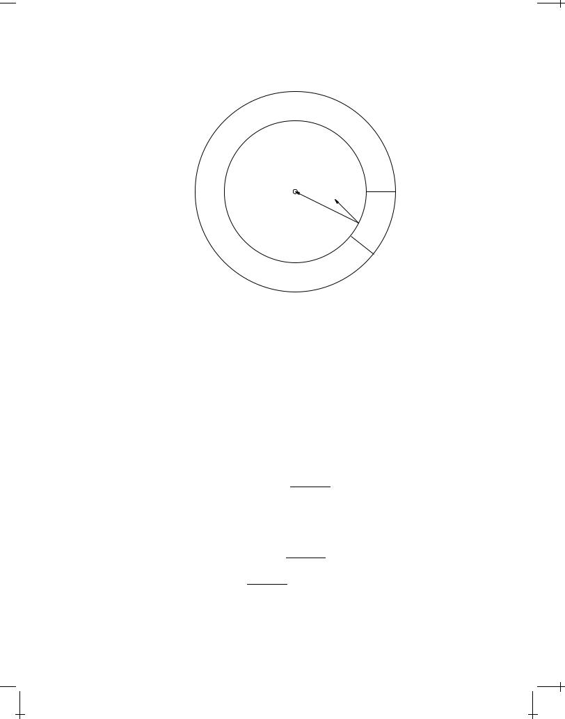
and consider a source region with such a limited spatial extent that the charges and currents are well localised. Specifically, we consider a charge q0, for instance an electron, which, classically, can be thought of as a localised, unstructured and rigid “charge distribution” with a small, finite radius. The part of this “charge distribution” dq0 which we are considering is located in dV0 = d3x0 in the sphere in Figure 8.5 on the following page. Since we assume that the electron (or any other other similar electric charge) is moving with a velocity v whose direction is arbitrary and whose magnitude can be almost comparable to the speed of light, we cannot say that the charge and current to be used in

(8.57) is V (tret0 ;x0)d3x0 and V v (tret0 ;x0)d3x0, respectively, because in the fi- nite time interval during which the observed signal is generated, part of the

charge distribution will “leak” out of the volume element d3x0.

x0(t0) q0

FIGURE 8.2: Signals which are observed at the field point x at time t were generated at source points x0(t0) on a sphere, centred on x and expanding, as time increases, with the velocity c outward from the centre. The source charge element moves with an arbitrary velocity v and gives rise to a source “leakage” out of the source volume dV0 = d3x0.

8.5.1 The Liénard-Wiechert potentials

The charge distribution in Figure 8.5 on page 112 which contributes to the field at x(t) is located at x0(t0) on a sphere with radius r = jx x0j = c(t t0).

The radius interval of this sphere from which radiation is received at the field point x during the time interval (t;t +dt) is (r;r +dr) and the net amount of charge in this radial interval is

where the last term represents the amount of “source leakage” due to the fact that the charge distribution moves with velocity v. Since dt =dr=c and dS dr = d3x0 we can rewrite this expression for the net charge as