

exploring-splunk
.pdfExploring Splunk
age. If you specify an optional by-clause of additional fields, the most frequent values for each distinct group of values of the by-clause fields are returned.
The opposite of top is rare
The opposite of the top command is the rare command. Sometimes you want to know what is the least common value for a field (instead of the most common). The rare command does exactly that.
Table 4-7. top Command Examples
Command |
Result |
… | top 20 url |
Return the 20 most common URLs. |
|
|
… | top 2 user by host |
Return the top 2 user values for each |
|
host. |
|
|
… | top user, host |
Return the top 10 (default) user- |
|
host combinations. |
|
|
The second example in Table 4-7, top 2 user by host, is illustrated in Figure 4-6.
host |
user |
< elds. . . > |
host-1 user_A |
. . .. |
|
host-1 user_A |
. . .. |
|
host-1 user_B |
. . .. |
|
host-1 user_C |
. . .. |
|
host-1 user_C |
. . .. |
|
host-1 user_C |
. . .. |
|
host-1 user_D |
. . .. |
|
host-2 user_E |
. . ... |
|
host-2 user_E |
. . .. |
|
host-2 |
user_F |
. . .. |
host-2 |
user_G |
. . .. |
host-2 |
user_G |
. . .. |
previous search results
...|
host |
user |
count |
percent |
host-1 user_A |
2 |
16.67 |
|
host-1 user_B |
1 |
8.33 |
|
host-1 |
user_C |
3 |
25.00 |
host-1 |
user_D |
1 |
8.33 |
host-2 |
|
2 |
16.67 |
user_F |
1 |
8.33 |
|
|
|
2 |
16.67 |
host |
user |
count |
percent |
host-1 user_C |
3 |
25.00 |
|
host-1 |
user_A |
2 |
16.67 |
host-2 |
user_E |
2 |
16.67 |
host-2 |
user_G |
2 |
16.67 |
intermediate results:
identifying count & nal results percent of “user” values
for each “host” value
top 2 user by host
Figure 4-6. top Command Example
42

Chapter 4: SPL: Search Processing Language
stats
The stats command calculates aggregate statistics over a dataset, similar to SQL aggregation. The resultant tabulation can contain one row, which represents the aggregation over the entire incoming result set, or a row for each distinct value of a specified by-clause.
There’s more than one command for statistical calculations. The stats, chart, and timechart commands perform the same statistical calculations on your data, but return slightly different result sets to enable you to more easily use the results as needed.
•The stats command returns a table of results where each row represents a single unique combination of the values of the group-by fields.
•The chart command returns the same table of results, with rows as any arbitrary field.
•The timechart command returns the same tabulated results, but the row is set to the internal field, _time, which enables you to chart your results over a time range.
Table 4-8 shows a few examples of using the stats command.
What “as” means
Note: The use of the keyword as in some of the commands in Table 4-14. as is used to rename a field. For example, sum(price) as “Revenue” means add up all the price fields and name the column showing the results “Revenue.”
Table 4-8. stats Command Examples
Command |
Result |
|
… | stats dc(host) |
Return the distinct count (i.e., |
|
|
unique) of host values. |
|
… | stats avg(kbps) by host |
Return the average transfer rate for |
|
|
each host. |
|
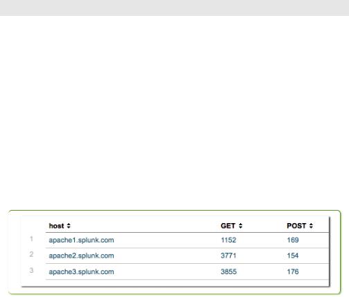
… | stats |
Return the number of different types |
|
count(eval(method=”GET”)) |
of requests for each Web server |
|
as GET, |
||
(host). The resultant table contains |
||
count(eval(method=”POST”)) as |
||
a row for each host and columns for |
||
POST by host |
||
the GET and POST request method |
||
|
||
|
counts. |
|
... | top limit=100 referer_ |
Return the total number of hits from |
|
domain | stats sum(count) as |
the top 100 values of referer_do- |
|
total |
||
main. |
||
|
43
Exploring Splunk
… | stats count, |
Using USGS Earthquakes data, return |
|
max(Magnitude), |
the number of quakes and additional |
|
min(Magnitude), |
||
statistics, for each Region. |
||
range(Magnitude), |
||
|
||
avg(Magnitude) by Region |
|
|
|
|
|
… | stats values(product_type) |
Return a table with Type, Name, and |
|
as Type, values(product_name) |
Revenue columns for each prod- |
|
as Name, sum(price) as “Rev- |
||
uct_id sold at a shop. Also, format |
||
enue” by product_id | re- |
||
the Revenue as $123,456. |
||
name product_id as “Prod- |
||
|
||
uct ID” | eval Revenue=”$ |
|
|
“.tostring(Revenue,”commas”) |
|
|
|
|
The third example in Table 4-8, retrieving the number of GET and POST requests per host, is illustrated in Figure 4-7.
Figure 4-7. stats Command Example
Table 4-9 lists statistical functions that you can use with the stats command. (These functions can also be used with the chart and timechart commands, which are discussed later.)
|
|
Table 4-9. stats Statistic al Functions |
|
|
|
|
|
|
|
|
Mathematical Calculations |
|
avg(X) |
|
Returns average of the values of field X; see also, |
|
|
|
mean(X). |
|
|
|
|
|
count(X) |
|
Returns the number of occurrences of the field X; to |
|
|
|
indicate a field value to match, format the X argument |
|
|
|
as an expression: eval(field="value"). |
|
|
|
|
|
dc(X) |
|
Returns the count of distinct values of field X. |
|
|
|
|
|
max(X) |
|
Returns the maximum value of field X. If the values are |
|
|
|
non-numeric, the max is determined per lexicographic |
|
|
|
ordering. |
|
|
|
|
|
median(X) |
|
Returns the middle-most value of field X. |
|
|
|
|
|
min(X) |
|
Returns the minimum value of field X. If the values are |
|
|
|
non-numeric, the min is determined per lexicographic |
|
|
|
ordering. |
|
|
|
|
|
|
|
|
44

|
|
Chapter 4: SPL: Search Processing Language |
|
|
|
|
|
|
|
|
|
|
mode(X) |
Returns the most frequent value of field X. |
|
|
|
|
|
|
perc<percent- |
Returns the <percent-num>-th value of field X; for |
|
|
num>(X) |
example, perc5(total) returns the 5th percentile value |
|
|
|
of the total field. |
|
|
|
|
|
|
range(X) |
Returns the difference between the max and min values |
|
|
|
of field X, provided values are numeric. |
|
|
|
|
|
|
stdev(X) |
Returns the sample standard deviation of field X. You |
|
|
|
can use wildcards when you specify the field name; |
|
|
|
for example, "*delay", which matches both "delay" and |
|
|
|
"xdelay". |
|
|
|
|
|
|
sum(X) |
Returns the sum of the values of field X. |
|
|
|
|
|
|
var(X) |
Returns the sample variance of field X. |
|
|
|
|
|
|
|
Value Selections |
|
|
first(X) |
Returns the first value of field X; opposite of last(X). |
|
|
|
|
|
|
last(X) |
Returns the last value of field X; opposite of first(X). |
|
|
|
Generally, a field’s last value is the most chronologically |
|
|
|
oldest value. |
|
|
|
|
|
|
list(X) |
Returns the list of all values of field X as a multivalue |
|
|
|
entry. The order of the values matches the order of input |
|
|
|
events. |
|
|
values(X) |
Returns a list (as a multivalue entry) of all distinct values |
|
|
|
of field X, ordered lexicographically. |
|
timechart only (not applicable to chart or stats)
per_day(X) |
Returns the rate of field X per day |
per_hour(X) |
Returns the rate of field X per hour |
per_minute(X) |
Returns the rate of field X per minute |
per_second(X) |
Returns the rate of field X per year |
Note: All functions except those in the timechart only category are applicable to the chart, stats, and timechart commands.
chart
The chart command creates tabular data output suitable for charting. You specify the x-axis variable using over or by.
Table 4-10 shows a few simple examples of using the chart command; for more realistic scenarios, see Chapter 6.
45

Exploring Splunk
Table 4-10. chart Command Examples
Command |
Result |
|
… | chart max(delay) over host |
Return max(delay) for each value of |
|
|
host. |
|
|
|
|
… | chart max(delay) by size |
Chart the maximum delay by size, |
|
bins=10 |
where size is broken down into a |
|
|
||
|
maximum of 10 equal-size buckets. |
|
|
|
|
… | chart eval(avg(size)/ |
Chart the ratio of the average (mean) |
|
max(delay)) as ratio by host |
size to the maximum delay for each |
|
user |
||
distinct host and user pair. |
||
|
||
|
|
|
... | chart dc(clientip) over |
Chart the number of unique cli- |
|
date_hour by category_id |
entip values per hour by category. |
|
usenull=f |
||
usenull=f excludes fields that don’t |
||
|
||
|
have a value. |
|
… | chart count over Magnitude |
Chart the number of earthquakes by |
|
by Region useother=f |
Magnitude and Region. Use the |
|
|
||
|
useother=f argument to not output |
|
|
an “other” value for rarer Regions. |
|
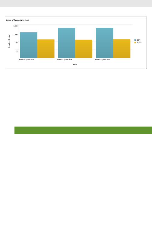
… | chart |
Chart the number of GET and POST |
|
count(eval(method=”GET”)) |
page requests that occurred for each |
|
as GET, |
||
Web server (host) |
||
count(eval(method=”POST”)) as |
||
|
||
POST by host |
|
|
|
|
Figures 4-8 (tabulated results) and 4-9 (bar chart on a logarithmic scale) illustrate the results of running the last example in Table 4-10:
Figure 4-8. chart Command Example—Tabulated Results
46
Chapter 4: SPL: Search Processing Language
Figure 4-9. chart Command Example—Report Builder Formatted Chart
timechart
The timechart command creates a chart for a statistical aggregation applied to a field against time as the x-axis.
Table 4-11 shows a few simple examples of using the timechart command. Chapter 6 offers more examples of using this command in context.
Table 4-11. timechart Command Example
Command |
Result |
… | timechart span=1m avg(CPU) |
Chart the average value of CPU usage |
by host |
each minute for each host. |
|
|
… | timechart span=1d count |
Chart the number of purchases made |
by product-type |
daily for each type of product. The |
|
|
|
span=1d argument buckets the count |
|
of purchases over the week into daily |
|
chunks. |
|
|
…| timechart avg(cpu_seconds) |
Chart the average cpu_seconds by |
by host | outlier |
host and remove outlying values that |
|
|
|
may distort the timechart’s y-axis. |
|
|
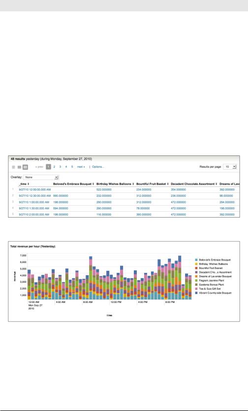
…| timechart per_hour(price) |
Chart hourly revenue for the prod- |
by product_name |
ucts that were purchased yesterday. |
|
|
|
The per_hour() function sums the |
|
values of the price field for each item |
|
(product_name) and scales that |
|
sum appropriately depending on the |
|
timespan of each bucket. |
|
|
47
Exploring Splunk
… | timechart |
Chart the number of page requests |
|
count(eval(method=”GET”)) |
over time. The count() function and |
|
as GET, |
||
eval expressions are used to count |
||
count(eval(method=”POST”)) as |
||
the different page request methods, |
||
POST |
||
GET and POST. |
||
|
||
|
|
|
… | timechart per_ |
For an ecommerce website, chart |
|
hour(eval(method=”GET”)) |
per_hour the number of produc t |
|
as Views, per_ |
||
views and purchases—answering |
||
hour(eval(action=”purchase”)) |
||
the question, how many views did |
||
as Purchases |
||
|
not lead to purchases? |
The fourth example in Table 4-11, charting hourly revenues by product name, is illustrated in figures 4-10 and 4-11.
Figure 4-10. timechart Command Example—Tabulated Results
Figure 4-11. timechart Command Example—Formatted Timechart
Filtering, Modifying, and Adding Fields
These commands help you get only the desired fields in your search results. You might want to simplify your results by using the fields command to remove some fields. You might want to make your field values
48

Chapter 4: SPL: Search Processing Language
more readable for a particular audience by using the replace command.
Or you might need to add new fields with the help of commands such as eval, rex, and lookup:
•The eval command calculates the value of a new field based on other fields, whether numerically, by concatenation, or through
Boolean logic.
•The rex command can be used to create new fields by using regular expressions to extracting patterned data in other fields.
•The lookup command adds fields based on looking at the value in an event, referencing a lookup table, and adding the fields in matching rows in the lookup table to your event.
These commands can be used to create new fields or they can be used to overwrite the values of existing fields. It’s up to you.
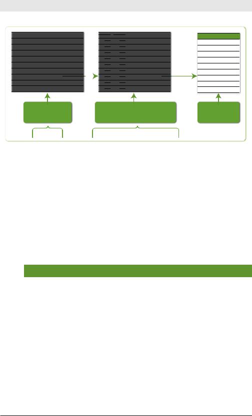
fields
The fields command removes fields from search results. Typical commands are shown in Table 4-6.
Table 4-12. fields Command Examples
Command |
Result |
… | fields – field1, field2 |
Remove field1 and field2 from |
|
the search results. |
|
|
… | fields field1 field2 |
Keep only field1 and field2. |
|
|
… | fields field1 error* |
Keep only field1 and all fields |
|
whose names begin with error. |
|
|
… | fields field1 field2 | |
Keep only field1 and field2 and |
fields - _* |
remove all internal fields (which |
|
|
|
begin with an underscore). (Note: |
|
Removing internal fields can cause |
|
Splunk Web to render results in- |
|
correctly and create other search |
|
problems.) |
|
|
The first example in Table 4-12, fields – field1, field2, is illustrated in Figure 4-12.
49
Exploring Splunk
eld1 |
eld1 |
eld1 |
< elds. . . > |
|
|
eld1 |
eld1 |
eld1 |
< elds. . . > |
1 |
A |
a |
. . . |
|
1 |
A |
a |
. . . |
|
2 |
B |
b |
. . . |
|
2 |
B |
b |
. . . |
|
3 |
C |
c |
. . . |
|
3 |
C |
c |
. . . |
|
4 |
D |
d |
. . . |
|
4 |
D |
d |
. . . |
|
5 |
E |
e |
. . . |
|
5 |
E |
e |
. . . |
|
6 |
F |
f |
. . . |
|
6 |
F |
f |
. . . |
|
7 |
G |
g |
. . . |
|
|
7 |
G |
g |
. . . |
|
|||||||||
8 |
H |
h |
. . . |
|
8 |
H |
h |
. . . |
|
9 |
I |
i |
. . . |
|
9 |
I |
i |
. . . |
|
eld1 < elds. . . >
a. . .
b. . .
c. . .
d. . .
e. . .
f. . .
g. . .
h. . .
i. . .
previous search results
...|
Key Points
remove eld1 and eld 2 |
nal results |
columns |
|
fields - field1 field2
Figure 4-12. fields Command Example
Internal fields, i.e., fields whose names start with an underscore, are unaffected by the fields command, unless explicitly specified.
replace
The replace command performs a search-and-replace of specified field values with replacement values.
The values in a search and replace are case-sensitive.
Table 4-13. replace Command Examples
Command |
Result |
replace *localhost with loc- |
Change any host value that ends |
alhost in host |
with localhost to localhost. |
|
|
|
|
replace 0 with Critical , 1 |
Change msg_level values of 0 to |
with Error in msg_level |
Critical, and change msg_level |
|
|
|
values of 1 to Error. |
|
|
replace aug with August in |
Change any start_month or end_ |
start_month end_month |
month value of aug to August. |
|
|
replace 127.0.0.1 with local- |
Change all field values of 127.0.0.1 |
host |
to localhost. |
|
The second example in Table 4-13, replace 0 with Critical , 1 with
Error in msg_level, is illustrated in Figure 4-13.
50

Chapter 4: SPL: Search Processing Language
msg_level |
< elds. . . > |
|
|
msg_level < elds. . . > |
|
0 |
. . . |
|
|
Critical |
. . . |
1 |
. . . |
|
|
Error |
. . . |
0 |
. . . |
|
|
Critical |
. . . |
0 |
. . . |
|
|
Critical |
. . . |
3 |
. . . |
|
3 |
. . . |
|
4 |
. . . |
|
4 |
. . . |
|
0 |
. . . |
|
|
Critical |
. . . |
|
|||||
3 |
. . . |
|
3 |
. . . |
|
1 |
. . . |
|
|
Error |
. . . |
previous |
nal results |
search results |
|
...| |
replace 0 with Critical, |
|
|
|
1 with Error in msg_level |
Figure 4-13. replace Command Example
eval
The eval command calculates an expression and puts the resulting value into a new field. The eval and where commands use the same expression syntax; Appendix E lists all the available functions.
Table 4-14. eval Command Examples
Command |
Result |
|
… | eval velocity=distance/ |
Set velocity to distance divided by |
|
time |
time. |
|
|
||
|
|
|
… | eval status = if(error == |
Set status to OK if error is 200; other- |
|
200, “OK”, “Error”) |
wise set status to Error. |
|
|
||
… | eval sum_of_areas = pi() |
Set sum_of_areas to be the sum of the |
|
* pow(radius_a, 2) + pi() * |
areas of two circles. |
|
pow(radius_b, 2) |
||
|
||
|
|
Figure 4-14 illustrates the first example in Table 4-14, eval velocity=distance/time.
51