MIMO III: diversity–multiplexing tradeoff and universal space-time codes
Exercise 9.6 Verify the claim in (9.28) by showing that the sum of the pairwise error probabilities in (9.26), with xA xB each a pair of QAM symbols (the union bound on the error probability) has a decay rate of 2 − r with increasing SNR.
Exercise 9.7 The result in Exercise 9.6 can be generalized. Show that the diversity gain of transmitting uncoded QAMs (each at a rate of R = r/n log SNR bits/s/Hz) on the n transmit antennas of an i.i.d. Rayleigh fading MIMO channel with n receive antennas is n − r.
Exercise 9.8 Consider the expression for poutmimo in (9.29) and for poutiid in (9.30). Suppose that the entries of the MIMO channel H have some joint distribution and are not necessarily i.i.d. Rayleigh.
1. Show that
poutiid r log SNR ≥ poutmimo r log SNR ≥ log det Inr + SNR HH < r log SNR (9.87)
2.Show that the lower bound above decays at the same polynomial rate as poutiid with increasing SNR.
3.Conclude that the polynomial decay rates of both poutmimo and poutiid with increasing SNR are the same.
Exercise 9.9 Consider a scalar slow fading channel
y m = hx m + w m
with an optimal diversity–multiplexing tradeoff d · , i.e.,
lim
log pout r log SNR
= −
d
r
log SNR
SNR→
Let > 0 and consider the following event on the channel gain h:
= h log 1 + h 2SNR1− < R
(9.88)
(9.89)
(9.90)
1.Show, by conditioning on the event or otherwise, that the probability of error pe SNR of QAM with rate R = r log SNR bits/symbol satisfies
lim
log pe SNR
d
log SNR ≤ −
r 1
−
(9.91)
SNR→
Hint: you should show that conditional on the not happening, the probability of error decays very fast and is negligible compared to the probability of error conditional on happening.
2.Hence, conclude that QAM achieves the diversity–multiplexing tradeoff of any scalar channel.
3.More generally, show that any constellation that satisfies the condition (9.38) achieves the diversity–multiplexing tradeoff curve of the channel.
4.Even more generally, show that any constellation that satisfies the condition
dmin2
> c ·
1
for any constant c > 0
(9.92)
2R
419
9.4 Exercises
achieves the diversity–multiplexing tradeoff curve of the channel. This shows that the condition (9.38) is really only an order-of-magnitude condition. A slightly weaker version of this condition is also necessary for a code to be approximately universal; see [118].
Exercise 9.10 Consider coding over a block length N for communication over the parallel channel in (9.17). Derive the universal code design criterion, generalizing the derivation in Section 9.2.2 over a block length of 1.
Exercise 9.11 In this exercise we will try to explicitly calculate the universal code design criterion for the parallel fading channel; for given differences between a pair of normalized codewords, the criterion is to maximize the expression in (9.49).
1.Suppose the codeword differences on all the sub-channels have the same magnitude, i.e., d1 = · · · = dL . Show that in this case the worst case channel is the same over all the sub-channels and the universal criterion in (9.49) simplifies considerably to
L 2R − 1 d1 2
(9.93)
2.Suppose the codeword differences are ordered: d1 ≤ · · · ≤ dL .
(a)Argue that if the worst case channel h on the th sub-channel is non-zero, then it is also non-zero on all the sub-channels 1 − 1.
(b)Consider the largest k such that
dk 2k ≤ 2RL d1 · · · dk 2 ≤ dk+1 2k
(9.94)
with dL+1 defined as + . Argue that the worst-case channel is zero on all the sub-channels k+1 L. Observe that k = L when all the codeword differences have the same magnitude; this is in agreement with the result in part (1).
3.Use the results of the previous part (and the notation of k from (9.94)) to derive an explicit expression for in (9.49):
k d1 · · · dk 2 = 2−RL
(9.95)
Conclude that the universal code design criterion is to maximize
k 2RL d1d2
· · · dk 2 1/k − k 1
d 2
(9.96)
=
Exercise 9.12 Consider the repetition code illustrated in Figure 9.12. This code is for the 2-parallel channel with R = 2 bits/s/Hz per sub-channel. We would like to evaluate the value of the universal design criterion, minimized over all pairs of codewords. Show that this value is equal to 8/3. Hint: The smallest value is yielded by choosing the pair of codewords as nearest neighbors in the QAM constellation. Since this is a repetition code, the codeword differences are the same for both the channels; now use (9.93) to evaluate the universal design criterion.
Exercise 9.13 Consider the permutation code illustrated in Figure 9.13 (with R = 2 bits/s/Hz per sub-channel). Show that the smallest value of the universal design criterion, minimized over all choices of codeword pairs, is equal to 44/9.
420
MIMO III: diversity–multiplexing tradeoff and universal space-time codes
Exercise 9.14 In this exercise we will explore the implications of the condition for approximate universality in (9.53).
1.Show that if a parallel channel scheme satisfies the condition (9.53), then it achieves the diversity–multiplexing tradeoff of the parallel channel. Hint: Do Exercise 9.9 first.
2.Show that the diversity–multiplexing tradeoff can still be achieved even when the scheme satisfies a more relaxed condition:
d1d2 · · · dL 2/L > c ·
1
for some constant c > 0
(9.97)
L2R
Exercise 9.15 Consider the class of permutatation codes for the L-parallel channel described in Section 9.2.2. The codeword is described as q 2q Lq where q belongs to a normalized QAM (so that each of the I and Q channels are peak constrained by ±1) with 2LR points; so, the rate of the code is R bits/s/Hz per sub-channel. In this exercise we will see that this class contains approximately universal codes.
1.Consider random permutations with the uniform measure; since there are 2LR! of them, each of the permutations occurs with probability 1/2LR!. Show that the average inverse product of the pairwise codeword differences, averaged over both the codeword pairs and the random permutations, is upper bounded as follows:
2 L
1
2LR 2LR − 1
≤ LLRL
× q
1
1
q
q1
−
q2
2
2
q1
−
2
q2
2
· · ·
Lq1
−
Lq2
2
=2
(9.98)
2. Conclude from the previous part that there exist permutations 2 L such that
1
1
1
2=1
−
−
· · ·
−
2LR
q
q
q
q1
q2
2
2q1
2q2
2
Lq1
Lq2
2
≤ LLRL2LR
(9.99)
3.Now suppose we fix q1 and consider the sum of the inverse product of all the possible pairwise codeword differences:
1
f q1 = q2=q1
q1 − q2 2 2q1 − 2q2 2 · · · Lq1 − Lq2 2
(9.100)
Since f q1 ≥ 0, argue from (9.99) that at least half the QAM points q1 must have the property that
f q1 ≤ 2LLRL2LR
(9.101)
Further, conclude that for such q1 (they make up at least half of the total QAM points) we must have for every q2 =q1 that
q1 − q2 2 2q1 − 2q2 2 · · · Lq1 − Lq2 2 ≥
1
(9.102)
2LLRL2LR
421
9.4 Exercises
4.Finally, conclude that there exists a permutation code that is approximately universal for the parallel channel by arguing the following:
•Expurgating no more than half the number of QAM points only reduces the total rate LR by no more than 1 bit/s/Hz and thus does not affect the multiplexing gain.
•The product distance condition on the permutation codeword differences in (9.102) does not quite satisfy the condition for approximate universality in (9.97). Relax the condition in (9.97) to
d1d2 · · · dL 2/L > c ·
1
for some constant c > 0
(9.103)
R2R
and show that this is sufficient for a code to achieve the optimal diversity– multiplexing tradeoff curve.
Exercise 9.16 Consider the bit-reversal scheme for the parallel channel described in Section 9.2.2. Strictly speaking, the condition in (9.57) is not true for every integer between 0 and 2R − 1. However, the set of integers for which this is not true is small (i.e., expurgating them will not change the multiplexing rate of the scheme). Thus the bit-reversal scheme with an appropriate expurgation of codewords is approximately universal for the 2-parallel channel. A reading exercise is to study [118] where the expurgated bit-reversal scheme is described in detail.
Exercise 9.17 Consider the bit-reversal scheme described in Section 9.2.2 but with every alternate bit flipped after the reversal. Then for every pair of normalized codeword differences, it can be shown that
d1d2 2 >
1
(9.104)
64 · 22R
where the data rate is R bits/s/Hz per sub-channel. Argue now that the bit-reversal scheme with alternate bit flipping is approximately universal for the 2-parallel channel. A reading exercise is to study the proof of (9.104) in [118]. Hint: Compare (9.104) with (9.53) and use the result derived in Exercise 9.14.
Exercise 9.18 Consider a MISO channel with the fading channels from the nt transmit antennas, h1 hnt , i.i.d.
1. Show that
log 1 +
SNR
nt
< r log SNR
h 2
(9.105)
nt
=
1
and
+ SNR h 2 < nt r log SNR
nt1 log 1
(9.106)
=
have the same decay rate with increasing SNR.
2.Interpret (9.105) and (9.106) with the outage probabilities of the MISO channel and that of a parallel channel obtained through an appropriate transformation of the MISO channel, respectively. Argue that the conversion of the MISO channel into a parallel channel discussed in Section 9.2.3 is approximately universal for the class of i.i.d. fading coefficients.
422
MIMO III: diversity–multiplexing tradeoff and universal space-time codes
Exercise 9.19 Consider an nt × nt matrix D. Show that
min h DD h
=
2
(9.107)
h h
=
1
1
where 1 is the smallest singular value of D.
Exercise 9.20 Consider the Alamouti transmit codeword (cf. (9.84)) with u1 u2 independent uncoded QAMs with 2R points in each.
1.For every codeword difference matrix
d1
− d2
(9.108)
d2
d1
show that the two singular values are the same and equal to
d1 2 + d2 2
.
2. With the codeword difference matrix normalized as in (9.68)
and each of the QAM
symbols u1 u2
constrained in power of SNR/2 (i.e., both the I and Q channels are
peak constrained by
± SNR/2), show that if the codeword difference d is not
zero, then it is
2
d 2 ≥
= 1 2
2R
3.Conclude from the previous steps that the square of the smallest singular value of the codeword difference matrix is lower bounded by 2/2R. Since the condition for approximate universality in (9.70) is an order-of-magnitude one (the constant factor next to the 2R term does not matter, see Exercises 9.9 and 9.14), we have explicitly shown that the Alamouti scheme with uncoded QAMs on the two streams is approximately universal for the two transmit antenna MISO channel.
Exercise 9.21 Consider the D-BLAST architecture in (9.77) with just two interleaved streams for the 2 × 2 i.i.d. Rayleigh fading MIMO channel. The two streams are
independently
coded at rate R
=
r log
SNR
bits/s/Hz each and composed of the pair
of codewords
xA
xB
for = 1 2. The two streams are coded using an approx-
imately
universal parallel channel code (say, the bit-reversal scheme described in
Section 9.2.2).
A union bound averaged over the Rayleigh MIMO channel can be used to show that the diversity gain obtained by each stream with joint ML decoding is 4 − 2r. A reading exercise is to study the proof of this result in [118].
Exercise 9.22 [67] Consider transmitting codeword matrices of length at least nt on the nt × nr MIMO slow fading channel at rate R bits/s/Hz (cf. (9.71)).
1.Show that the pairwise error probability between two codeword matrices XA and XB, conditioned on a specific realization of the MIMO channel H, is
Q
SNR
HD 2
(9.109)
2
where D is the normalized codeword difference matrix (cf. (9.68)).
423
9.4 Exercises
2.Writing the SVDs H = U1 V1 and D = U2 V2 , show that the pairwise error probability in (9.109) can be written as
Q
SNR
V1 U2 2
(9.110)
2
3.Suppose the singular values are increasingly ordered in and decreasingly ordered in . For fixed U2, show that the channel eigendirections V1 that minimize the pairwise error probability in (9.110) are
V1 = U2
(9.111)
4.Observe that the channel outage condition depends only on the singular values of H (cf. Exercise 9.8). Use the previous parts to conclude that the calculation of the worst-case pairwise error probability for the MIMO channel reduces to the optimization problem
SNR
L
2
2
min
(9.112)
1 nmin 2
=1
subject to the constraint
1 +
SNR
≥ R
nmin
2
1 log
(9.113)
=
nt
Here we have written
= diag 1 nmin
and = diag 1 nt
5.Observe that the optimization problem in (9.112) and the constraint (9.113) are very similar to the corresponding ones in the parallel channel (cf. (9.43) and (9.40), respectively). Thus the universal code design criterion for the MIMO channel is the same as that of a parallel channel (cf. (9.47)) with the following parameters:
•there are nmin sub-channels,
•the rate per sub-channel is R/nmin bits/s/Hz,
•the parallel channel coefficients are 1 nmin , the singular values of the MIMO channel, and
•the codeword differences are the smallest singular values, 1 nmin , of the codeword difference matrix.
Exercise 9.23 Using the analogy between the worst-case pairwise error probability of a MIMO channel and that of an appropriately defined parallel channel (cf. Exercise 9.22), justify the condition for approximate universality for the MIMO channel in (9.79).
Exercise 9.24 Consider transmitting codeword matrices of length l ≥ nt on the nt × nr MIMO slow fading channel. The total power constraint is SNR, so for any transmit codeword matrix X, we have X 2 ≤ lSNR. For a pair of codeword matrices XA and XB, let the normalized codeword difference matrix be D (normalized as in (9.68)).
424
MIMO III: diversity–multiplexing tradeoff and universal space-time codes
1. Show that D satisfies
2
D 2 ≤
XA 2
+ XB 2 ≤ 4l
(9.114)
SNR
2. Writing the singular values of D as 1 nt , show that
nt
2 ≤ 4l
(9.115)
=1
Thus, each of the singular values is upper bounded by 2√l, a constant that does
not increase with SNR.
Exercise 9.25 [152] Consider the following transmission scheme (spanning two sym-
bols) for the two transmit antenna MIMO channel. The entries of the transmit codeword
matrix X = xij are defined as
x11
u1
x21
u3
x22 = R 1
u2
and
x12 = R 2
u4
(9.116)
Here u1 u2 u3 u4 are independent QAMs of size 2R/2 each (so the data rate of this scheme is R bits/s/Hz). The rotation matrix R is (cf. (3.46))
cos
sin
R = sin
− cos
(9.117)
With the choice of the angles 1 2 equal to 1/2 tan−1 2 and 1/2 tan−1 1/2 radians respectively, Theorem 2 of [152] shows that the determinant of every normalized codeword difference matrix D satisfies
det D 2 ≥
1
(9.118)
10 · 2R
Conclude that the code described in (9.116), with the appropriate choice of the angles1 2 above, is approximately universal for every MIMO channel with two transmit antennas.
C H A P T E R
10 MIMO IV: multiuser communication
In Chapters 8 and 9, we have studied the role of multiple transmit and receive antennas in the context of point-to-point channels. In this chapter, we shift the focus to multiuser channels and study the role of multiple antennas in both the uplink (many-to-one) and the downlink (one-to-many). In addition to allowing spatial multiplexing and providing diversity to each user, multiple antennas allow the base-station to simultaneously transmit or receive data from multiple users. Again, this is a consequence of the increase in degrees of freedom from having multiple antennas.
We have considered several MIMO transceiver architectures for the point- to-point channel in Chapter 8. In some of these, such as linear receivers with or without successive cancellation, the complexity is mainly at the receiver. Independent data streams are sent at the different transmit antennas, and no cooperation across transmit antennas is needed. Equating the transmit antennas with users, these receiver structures can be directly used in the uplink where the users have a single transmit antenna each but the base-station has multiple receive antennas; this is a common configuration in cellular wireless systems.
It is less apparent how to come up with good strategies for the downlink, where the receive antennas are at the different users; thus the receiver structure has to be separate, one for each user. However, as will see, there is an interesting duality between the uplink and the downlink, and by exploiting this duality, one can map each receive architecture for the uplink to a corresponding transmit architecture for the downlink. In particular, there is an interesting precoding strategy, which is the “transmit dual” to the receiver-based successive cancellation strategy. We will spend some time discussing this.
The chapter is structured as follows. In Section 10.1, we first focus on the uplink with a single transmit antenna for each user and multiple receive antennas at the base-station. We then, in Section 10.2, extend our study to the MIMO uplink where there are multiple transmit antennas for each user. In Sections 10.3 and 10.4, we turn our attention to the use of multiple antennas in the downlink. We study precoding strategies that achieve the capacity of
425
426 MIMO IV: multiuser communication
the downlink. We conclude in Section 10.5 with a discussion of the system implications of using MIMO in cellular networks; this will link up the new insights obtained here with those in Chapters 4 and 6.
10.1 Uplink with multiple receive antennas
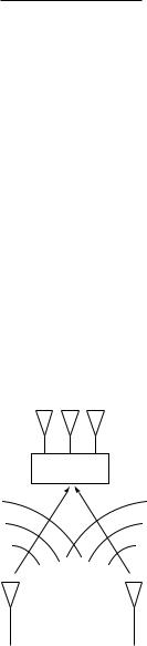
We begin with the narrowband time-invariant uplink with each user having a single transmit antenna and the base-station equipped with an array of antennas (Figure 10.1). The channels from the users to the base-station are time-invariant. The baseband model is
K
ym =
hkxkm + wm
(10.1)
k=1
with ym being the received vector (of dimension nr, the number of receive antennas) at time m, and hk the spatial signature of user k impinged on the receive antenna array at the base-station. User k’s scalar transmit symbol at time m is denoted by xkm and wm is i.i.d. 0 N0Inr noise.
10.1.1 Space-division multiple access
Figure 10.1 The uplink with single transmit antenna at each user and multiple receive antennas at the base-station.
In the literature, the use of multiple receive antennas in the uplink is often called space-division multiple access (SDMA): we can discriminate amongst the users by exploiting the fact that different users impinge different spatial signatures on the receive antenna array.
An easy observation we can make is that this uplink is very similar to the MIMO point-to-point channel in Chapter 5 except that the signals sent out on the transmit antennas cannot be coordinated. We studied precisely such a signaling scheme using separate data streams on each of the transmit antennas in Section 8.3. We can form an analogy between users and transmit antennas (so nt, the number of transmit antennas in the MIMO point-to-point channel in Section 8.3, is equal to the number of users K). Further, the equivalent MIMO point-to-point channel H is h1 hK , constructed from the SIMO channels of the users.
Thus, the transceiver architecture in Figure 8.1 in conjunction with the receiver structures in Section 8.3 can be used as an SDMA strategy. For example, each of the user’s signal can be demodulated using a linear decorrelator or an MMSE receiver. The MMSE receiver is the optimal compromise between maximizing the signal strength from the user of interest and suppressing the interference from the other users. To get better performance, one can also augment the linear receiver structure with successive cancellation to yield the MMSE–SIC receiver (Figure 10.2). With successive cancellation, there is also a further choice of cancellation ordering. By choosing a
427 10.1 Uplink with multiple receive antennas
MMSE
Decode
User 1
Receiver 1
User 1
y[m]
User 2
Subtract
MMSE
Decode
User 1
Receiver 2
User 2
Figure 10.2 The MMSE–SIC receiver: user 1’s data is first decoded and then the corresponding transmit signal is subtracted off before the next stage. This receiver structure, by changing the ordering of cancellation, achieves the two corner points in the capacity region.
different order, users are prioritized differently in the sharing of the common resource of the uplink channel, in the sense that users canceled later are treated better.
Provided that the overall channel matrix H is well-conditioned, all of these SDMA schemes can fully exploit the total number of degrees of freedom min K nr of the uplink channel (although, as we have seen, different schemes have different power gains). This translates to being able to simultaneously support multiple users, each with a data rate that is not limited by interference. Since the users are geographically separated, their transmit signals arrive in different directions at the receive array even when there is limited scattering in the environment, and the assumption of a wellconditioned H is usually valid. (Recall Example 7.4 in Section 7.2.4.) Contrast this to the point-to-point case when the transmit antennas are co-located, and a rich scattering environment is needed to provide a well-conditioned channel matrix H.
Given the power levels of the users, the achieved SINR of each user can be computed for the different SDMA schemes using the formulas derived in Section 8.3 (Exercise 10.1). Within the class of linear receiver architecture, we can also formulate a power control problem: given target SINR requirements for the users, how does one optimally choose the powers and linear filters to meet the requirements? This is similar to the uplink CDMA power control problem described in Section 4.3.1, except that there is a further flexibility in the choice of the receive filters as well as the transmit powers. The first observation is that for any choice of transmit powers, one always wants to use the MMSE filter for each user, since that choice maximizes the SINR for every user. Second, the power control problem shares the basic monotonicity property of the CDMA problem: when a user lowers its transmit power, it creates less interference and benefits all other users in the system. As a consequence, there is a component-wise optimal solution for the powers, where every user is using the minimum possible power to support the SINR requirements. (See Exercise 10.2.) A simple distributed power control algorithm will converge to the optimal solution: at each step, each user first updates its MMSE filter as a function of the current power levels of the other users, and then updates its own transmit power so that its SINR requirement is just met. (See Exercise 10.3.)