

Fundamentals Of Wireless Communication
.pdf388 |
MIMO III: diversity–multiplexing tradeoff and universal space-time codes |
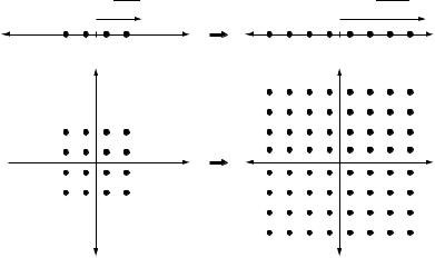
Figure 9.1 Tradeoff curves for the single antenna slow fading
Rayleigh channel. Fixed rate (0, 1)
|
(r) |
|
|
|
|
|
* |
|
|
|
|
|
Gaind |
|
|
|
|
|
Diversity |
QAM |
|
|
|
|
|
|
|
||
|
PAM |
|
|
Fixed reliability |
|
|
|
|
|
|
|
|
|
(1/2, 0) |
(1, 0) |
|
|
|
Spatial multiplexing gain r = R / log SNR |
|
|||
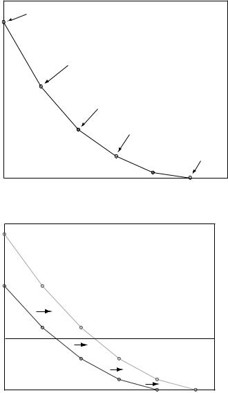
Figure 9.2 Increasing the SNR |
≈ |
√ |
SNR |
1 |
≈ 4SNR |
by 6dB decreases the error |
|
|
pe ↓ 4 |
√ |
|
PAM |
|
|
|
||
probability by 1/4 for both |
|
|
|
|
|
PAM and QAM due to a doubling of the minimum distance.
pe ↓ 14
QAM 
This is consistent with our observation in Section 3.1.3 that PAM uses only half the degrees of freedom of QAM. The increase in data rate is due to the packing of more constellation points for a given Dmin. This is illustrated in Figure 9.3.
The two endpoints represent two extreme ways of using the increase in the resource (SNR): increasing the reliability for a fixed data rate, or increasing the data rate for a fixed reliability. More generally, we can simultaneously increase the data rate (positive multiplexing gain r) and increase the reliability (positive diversity gain d > 0) but there is a tradeoff between how much of each type of gain we can get. The diversity–multiplexing curve describes this tradeoff. Note that the classical diversity gain only describes the rate of decay of the error probability for a fixed data rate, but does not provide any information on how well a scheme exploits the available degrees of freedom. For example, PAM and QAM have the same classical diversity
389 |
9.1 Diversity–multiplexing tradeoff |
|
|
Figure 9.3 Increasing the SNR |
≈ √SNR |
≈ √4 SNR |
|
by 6dB increases the data rate |
|||
PAM |
+1 bit |
||
for QAM by 2 bits/s/Hz but |
|
||
only increases the data rate of |
|
|
|
PAM by 1 bit/s/Hz. |
|
|
+2 bits
QAM 
gain, even though clearly QAM is more efficient in exploiting the available degrees of freedom. The tradeoff curve, by treating error probability and data rate in a symmetrical manner, provides a more complete picture. We see that in terms of their tradeoff curves, QAM is indeed superior to PAM (see Figure 9.1).
Optimal tradeoff
So far, we have considered the tradeoff between diversity and multiplexing in the context of two specific schemes: uncoded PAM and QAM. What is the fundamental diversity–multiplexing tradeoff of the scalar channel itself? For
the slow fading Rayleigh channel, the outage probability at a target data rate R = r log SNR is
pout = log 1 |
+ h 2SNR < r log SNR |
|||||||
|
|
h |
2 |
< |
SNRr − 1 |
|
||
= |
|
|
|
|
|
|
|
|
|
|
|
|
SNR |
||||
≈ |
1 |
|
|
|
|
|
(9.15) |
|
|
|
|
|
|||||
|
SNR1−r |
|
|
|
||||
at high SNR. In the last step, we used the fact that for Rayleigh fading,h 2 < ≈ for small . Thus
d r = 1 − r |
r 0 1 |
(9.16) |
Hence, the uncoded QAM scheme trades off diversity and multiplexing gains optimally.
The tradeoff between diversity and multiplexing gains can be viewed as a coarser way of capturing the fundamental tradeoff between error probability and data rate over a fading channel at high SNR. Even very simple,
390 MIMO III: diversity–multiplexing tradeoff and universal space-time codes
low-complexity schemes can trade off optimally in this coarser context (the uncoded QAM achieved the tradeoff for the Rayleigh slow fading channel). To achieve the exact tradeoff between outage probability and data rate, we need to code over long block lengths, at the expense of higher complexity.
9.1.3 Parallel Rayleigh channel
Consider the slow fading parallel channel with i.i.d. Rayleigh fading on each sub-channel:
y m = h x m + w m = 1 L |
(9.17) |
Here, the w are i.i.d. 0 1 additive noise and the transmit power per sub-channel is constrained by SNR. We have seen that L Rayleigh faded subchannels provide a (classical) diversity gain equal to L (cf. Section 3.2 and Section 5.4.4): this is an L-fold improvement over the basic single antenna slow fading channel. In the parlance we introduced in the previous section, this says that d 0 = L. How about the diversity gain at any positive multiplexing rate?
Suppose the target data rate is R = r log SNR bits/s/Hz per sub-channel. The optimal diversity d r can be calculated from the rate of decay of the outage probability with increasing SNR. For the i.i.d. Rayleigh fading parallel channel, the outage probability at rate per sub-channel R = r log SNR is (cf. (5.83))
|
+ h 2SNR < Lr log SNR |
|
|
pout = L |
1 log 1 |
(9.18) |
|
= |
|
|
|
Outage typically occurs when each of the sub-channels cannot support the rate R (Exercise 9.1): so we can write
pout ≈ |
log 1 + h1 2SNR < r log SNR L ≈ |
1 |
|
(9.19) |
SNRL1−r |
So, the optimal diversity–multiplexing tradeoff for the parallel channel with
L diversity branches is
d r = L 1 − r |
r 0 1 |
(9.20) |
an L-fold gain over the scalar single antenna performance (cf. (9.16)) at every multiplexing gain r; this performance is illustrated in Figure 9.4.
One particular scheme is to transmit the same QAM symbol over the L sub-channels; the repetition converts the parallel channel into a scalar channel with squared amplitude h 2, but with the rate reduced by a factor of 1/L.

394 |
MIMO III: diversity–multiplexing tradeoff and universal space-time codes |
(cf. 3.92). Each codeword is a pair of QAM symbols transmitted on the two antennas, and hence the distance between the two closest codewords is that between two adjacent constellation points in one of the QAM constellation, i.e., xA and xB differ only in one of the two QAM symbols. With a total data rate of R bits/s/Hz, each QAM symbol carries R/2 bits, and hence each of the I and Q channels carries R/4 bits. The distance between two adjacent constellation points is of the order of 1/2R/4. Thus, the worst-case pairwise error probability is of the order
16 · 2R |
|
16 |
|
SNR− 2−r |
(9.27) |
|
SNR2 = |
· |
|||||
|
|
|
||||
where the data rate R = r log SNR. This is the worst-case pairwise error probability, but Exercise 9.6 shows that the overall error probability is also of the same order. Hence, the diversity–multiplexing tradeoff of V-BLAST with ML decoding is
d r = 2 − r |
r 0 2 |
(9.28) |
As already remarked in Section 3.3.3, the (classical) diversity gain and the degrees of freedom utilized are not always sufficient to say which scheme is best. For example, the Alamouti scheme has a higher (classical) diversity gain than V-BLAST but utilizes fewer degrees of freedom. The tradeoff curves, in contrast, provide a clear basis for the comparison. We see that which scheme is better depends on the target diversity gain (error probability) of the operating point: for smaller target diversity gains, V-BLAST is better than the Alamouti scheme, while the situation reverses for higher target diversity gains.
Optimal tradeoff
Do any of the four schemes actually achieve the optimal tradeoff of the 2 × 2 channel? The tradeoff curve of the 2×2 i.i.d. Rayleigh fading MIMO channel turns out to be piecewise linear joining the points (0, 4), (1, 1) and (2, 0) (also shown in Figure 9.6). Thus, all of the schemes are tradeoff-suboptimal, except for V-BLAST with ML, which is optimal but only for r > 1.
The endpoints of the optimal tradeoff curve are (0, 4) and (2, 0), consistent with the fact that the 2 × 2 MIMO channel has a maximum diversity gain of 4 and 2 degrees of freedom. More interestingly, unlike all the tradeoff curves we have computed before, this curve is not a line but piecewise linear, consisting of two linear segments. V-BLAST with ML decoding sends two symbols per symbol time with (classical) diversity of 2 for each symbol, and achieves the gentle part, 2 − r, of this curve. But what about the steep part, 4 − 3r? Intuitively, there should be a scheme that sends 4 symbols over 3 symbol times (with a rate of 4/3 symbols/s/Hz)
395 9.1 Diversity–multiplexing tradeoff
and achieves the full diversity gain of 4. We will see such a scheme in Section 9.2.4.
9.1.6 nt × nr MIMO i.i.d. Rayleigh channel
Optimal tradeoff
Consider the nt × nr MIMO channel with i.i.d. Rayleigh faded gains. The optimal diversity gain at a data rate r log SNR bits/s/Hz is the rate at which the outage probability (cf. (8.81)) decays with SNR:
poutmimo r log SNR = |
min |
log det Inr +HKxH < r log SNR (9.29) |
|
Kx Tr Kx ≤SNR |
|
While the optimal covariance matrix Kx depends on the SNR and the data rate, we argued in Section 8.4 that the choice of Kx = SNR/ntInt is often used as a good approximation to the actual outage probability. In the coarser scaling of the tradeoff curve formulation, that argument can be made precise: the decay rate of the outage probability in (9.29) is the same as when the covariance matrix is the scaled identity. (See Exercise 9.8.) Thus, for the purpose of identifying the optimal diversity gain at a multiplexing rate r it suffices to consider the expression in (8.85):
poutiid r log SNR = |
log det Inr + |
SNR |
HH < r log SNR |
(9.30) |
|
||||
nt |
By analyzing this expression, the diversity–multiplexing tradeoff of the nt ×nr i.i.d. Rayleigh fading channel can be computed. It is the piecewise linear curve joining the points
k nt − k nr − k k = 0 nmin |
(9.31) |
as shown in Figure 9.7.
The tradeoff curve summarizes succinctly the performance capability of the slow fading MIMO channel. At one extreme where r → 0, the maximal diversity gain nt ·nr is achieved, at the expense of very low multiplexing gain. At the other extreme where r → nmin, the full degrees of freedom are attained. However, the system is now operating very close to the fast fading capacity and there is little protection against the randomness of the slow fading channel; the diversity gain is approaching 0. The tradeoff curve bridges between the two extremes and provides a more complete picture of the slow fading performance capability than the two extreme points. For example, adding one transmit and one receive antenna to the system increases the degrees of freedom min nt nr by 1; this corresponds to increasing the maximum possible multiplexing gain by 1. The tradeoff curve gives a more refined picture of the system benefit: for any diversity requirement d, the supported multiplexing gain is increased by 1.
 h
h