Fundamentals Of Wireless Communication
.pdf
309 |
7.3 Modeling of MIMO fading channels |
will have to be many wavelengths to be able to exploit this spatial multiplexing effect.
Summary 7.1 Multiplexing capability of MIMO channels
SIMO and MISO channels provide a power gain but no degree-of-freedom gain.
Line-of-sight MIMO channels with co-located transmit antennas and co-located receive antennas also provide no degree-of-freedom gain.
MIMO channels with far-apart transmit antennas having angular separation greater than 1/Lr at the receive antenna array provide an effective degree- of-freedom gain. So do MIMO channels with far-apart receive antennas having angular separation greater than 1/Lt at the transmit antenna array.
Multipath MIMO channels with co-located transmit antennas and co-located receive antennas but with scatterers/reflectors far away also provide a degree-of-freedom gain.
7.3 Modeling of MIMO fading channels
The examples in the previous section are deterministic channels. Building on the insights obtained, we migrate towards statistical MIMO models which capture the key properties that enable spatial multiplexing.
7.3.1 Basic approach
In the previous section, we assessed the capacity of physical MIMO channels by first looking at the rank of the physical channel matrix H and then its condition number. In the example in Section 7.2.4, for instance, the rank of H is 2 but the condition number depends on how the angle between the two spatial signatures compares to the spatial resolution of the antenna array. The two-step analysis process is conceptually somewhat awkward. It suggests that physical models of the MIMO channel in terms of individual multipaths may not be at the right level of abstraction from the point of view of the design and analysis of communication systems. Rather, one may want to abstract the physical model into a higher-level model in terms of spatially resolvable paths.
We have in fact followed a similar strategy in the statistical modeling of frequency-selective fading channels in Chapter 2. There, the modeling is directly on the gains of the taps of the discrete-time sampled channel rather than on the gains of the individual physical paths. Each tap can be thought
312 MIMO I: spatial multiplexing and channel modeling
onto the receive antenna array is along the unit spatial signature er%, given by (7.57). Recall (cf. (7.35))
|
|
|
|
|
|
|
|
1 |
|
|
|
|
|
|
|
sinLr% |
|
|
|
|
|||
|
fr% = er 0 er% = |
|
exp j r% nr |
− 1 |
|
|
|
(7.59) |
|||||||||||||||
|
nr |
sinLr%/nr |
|
||||||||||||||||||||
analyzed in Section 7.2.4. In particular, we have |
|
|
|
|
|
|
|
||||||||||||||||
|
r |
Lr = |
|
r |
Lr |
= |
|
r |
Lr |
|
|
|
= |
|
r |
− |
|
|
|||||
f |
|
|
k |
0 andf |
|
|
−k |
|
|
|
f |
|
nr − k |
|
k |
|
1 n |
|
|
|
1 |
(7.60) |
|
|
|
|
|
|
|
|
|
|
|
|
|
|
|
||||||||||
(Figure 7.5). Hence, the nr fixed vectors:
r |
|
= |
r |
|
r |
Lr |
|
r |
Lr |
|
|
|
|
e |
0 e |
|
1 |
e |
|
nr − 1 |
(7.61) |
|
|
|
|
|
|
form an orthonormal basis for the received signal space nr . This basis provides the representation of the received signals in the angular domain.
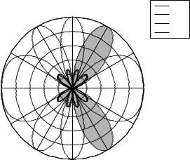
Why is this representation useful? Recall that associated with each vector er% is its beamforming pattern (see Figures 7.6 and 7.7 for examples). It has one or more pairs of main lobes of width 2/Lr and small side lobes. The different basis vectors erk/Lr have different main lobes. This implies that the received signal along any physical direction will have almost all of its energy along one particular erk/Lr vector and very little along all the others. Thus, this orthonormal basis provides a very simple (but approximate) decomposition of the total received signal into the multipaths received along the different physical directions, up to a resolution
of 1/Lr.
We can similarly define the angular domain representation of the transmitted signal. The signal transmitted at a direction % is along the unit vector et%, defined in (7.58). The nt fixed vectors:
t |
|
= |
t |
|
t |
Lt |
|
t |
|
|
Lt |
|
|
|
|
e |
0 e |
|
1 |
e |
|
|
nt |
− 1 |
(7.62) |
|
|
|
|
|
|
|
|
form an orthonormal basis for the transmitted signal space nt . This basis provides the representation of the transmitted signals in the angular domain. The transmitted signal along any physical direction will have almost all its energy along one particular etk/Lt vector and very little along all the others. Thus, this orthonormal basis provides a very simple (again, approximate)
313 |
7.3 Modeling of MIMO fading channels |
|
|
|
|
|
|
|
|
|
|
|||||||||
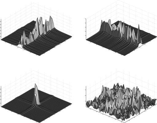
Figure 7.12 Receive |
120 |
90 |
1 |
60 |
|
120 |
90 |
1 |
60 |
|
120 |
90 |
1 |
|
120 |
90 |
1 |
60 |
|
|
|
|
|
|
|
||||||||||||||||
beamforming patterns of the |
|
|
|
|
|
|
|
|
60 |
|
|
|
|
|||||||
150 |
0.5 |
30 |
150 |
|
0.5 30 |
150 |
0.5 |
30 |
150 |
0.5 |
30 |
|||||||||
angular basis vectors. |
|
|||||||||||||||||||
|
|
|
|
|
|
|
|
|
|
|
|
|
|
|
|
|
|
|
|
|
Independent of the antenna |
180 |
|
|
|
0 |
180 |
|
|
|
0 |
180 |
|
|
|
0 |
180 |
|
|
|
0 |
spacing, the beamforming |
210 |
|
|
|
330 |
210 |
|
|
|
330 |
210 |
|
|
|
330 |
210 |
|
|
|
330 |
patterns all have the same |
240 |
270 300 |
240 |
270 |
|
300 |
240 |
270 |
|
300 |
240 |
270 300 |
||||||||
beam widths for the main |
|
|
|
|
|
|
|
|
|
|
|
|
|
|
|
|
|
|
|
|
lobe, but the number of main |
|
|
|
|
|
|
|
(a) L r = 2, n r = 4 |
|
|
|
|
|
|
|
|
|
|||
lobes depends on the spacing. |
|
|
|
|
|
|
|
|
|
|
|
|
|
|
|
|
|
|
|
|
(a) Critically spaced case; (b) |
|
|
|
|
|
|
90 |
1 |
|
|
|
90 |
1 |
|
|
|
|
|
|
|
Sparsely spaced case. (c) |
|
|
|
|
|
120 |
60 |
|
120 |
|
|
|
|
|
|
|
||||
|
|
|
|
|
|
|
|
|
60 |
|
|
|
|
|
|
|||||
Densely spaced case. |
|
|
|
|
|
150 |
0.5 |
30 |
150 |
0.5 |
30 |
|
|
|
|
|
||||
|
|
|
|
|
|
180 |
|
|
|
0 |
180 |
|
|
|
0 |
|
|
|
|
|
|
|
|
|
|
|
210 |
|
|
|
330 |
210 |
|
|
|
330 |
|
|
|
|
|
|
|
|
|
|
|
240 |
270 |
|
300 |
240 |
270 |
|
300 |
|
|
|
|
|
||
|
|
|
|
|
|
|
|
(b) L r = 2, n r = 2 |
|
|
|
|
|
|
|
|
|
|||
|
120 |
90 |
1 |
60 |
|
120 |
90 |
1 |
60 |
|
120 |
90 |
1 |
60 |
|
120 |
90 |
1 |
60 |
|
|
|
|
|
|
|
|
|
|
|
|
|
|
||||||||
|
150 |
0.5 |
30 |
150 |
|
0.5 |
30 |
150 |
0.5 |
30 |
150 |
0.5 |
30 |
|||||||
|
180 |
|
|
|
0 |
180 |
|
|
|
0 |
180 |
|
|
|
0 |
180 |
|
|
|
0 |
|
210 |
|
|
|
330 |
210 |
|
|
|
330 |
210 |
|
|
|
330 |
210 |
|
|
|
330 |
|
240 |
270 |
|
300 |
240 |
270 |
|
300 |
240 |
270 |
|
300 |
240 |
270 |
|
300 |
||||
|
120 |
90 |
1 |
60 |
|
120 |
90 |
1 |
60 |
|
120 |
90 |
1 |
60 |
|
120 |
90 |
1 |
60 |
|
|
|
|
|
|
|
|
|
|
|
|
|
|
||||||||
|
150 |
0.5 |
30 |
150 |
0.5 |
30 |
150 |
0.5 |
30 |
150 |
0.5 |
30 |
||||||||
|
180 |
|
|
|
0 |
180 |
|
|
|
0 |
180 |
|
|
|
0 |
180 |
|
|
|
0 |
|
210 |
|
|
|
330 |
210 |
|
|
|
330 |
210 |
|
|
|
330 |
210 |
|
|
|
330 |
|
240 |
270 |
|
300 |
240 |
270 |
|
300 |
240 |
270 |
|
300 |
240 |
270 |
|
300 |
||||
(c) L r = 2, n r = 8
decomposition of the overall transmitted signal into the components transmitted along the different physical directions, up to a resolution of 1/Lt.
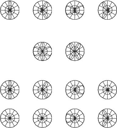
Examples of angular bases
Examples of angular bases, represented by their beamforming patterns, are shown in Figure 7.12. Three cases are distinguished:
•Antennas are critically spaced at half the wavelength ( r = 1/2). In this
case, each basis vector er k/Lr has a single pair of main lobes around the angles ± arccos k/Lr .
•Antennas are sparsely spaced ( r > 1/2). In this case, some of the basis vectors have more than one pair of main lobes.
•Antennas are densely spaced ( r < 1/2). In this case, some of the basis vectors have no main lobes.
314 |
MIMO I: spatial multiplexing and channel modeling |
These statements can be understood from the fact that the function fr %r is periodic with period 1/ r. The beamforming pattern of the vector er k/Lr is the polar plot
|
7 |
|
|
|
k |
7 |
|
|
|
7 |
|
|
|
|
7 |
|
|
|
7fr |
cos |
− |
Lr |
7 |
(7.63) |
||
|
7 |
|
|
|
|
7 |
|
|
and the main lobes are at all angles for which |
|
|||||||
cos = |
k |
mod |
1 |
|
(7.64) |
|||
|
|
|
||||||
Lr |
r |
|||||||
In the critically spaced case, 1/ r = 2 and k/Lr is between 0 and 2; there is a unique solution for cos in (7.64). In the sparsely spaced case, 1/ r < 2 and for some values of k there are multiple solutions: cos = k/Lr + m/ r for integers m. In the densely spaced case, 1/ r > 2, and for k satisfying Lr < k < nr − Lr, there is no solution to (7.64). These angular basis vectors do not correspond to any physical directions.
Only in the critically spaced antennas is there a one-to-one correspondence between the angular windows and the angular basis vectors. This case is the simplest and we will assume critically spaced antennas in the subsequent discussions. The other cases are discussed further in Section 7.3.7.
Angular domain transformation as DFT
Actually the transformation between the spatial and angular domains is a familiar one! Let Ut be the nt × nt unitary matrix the columns of which are the basis vectors in t. If x and xa are the nt-dimensional vector of transmitted signals from the antenna array and its angular domain representation respectively, then they are related by
x = Utxa xa = Ut x |
(7.65) |
Now the k l th entry of Ut is
1 |
exp |
j2 kl |
|
|
|
|
√ |
|
− |
k l = 0 nr − 1 |
(7.66) |
||
|
nt |
|||||
nt |
||||||
Hence, the angular domain representation xa is nothing but the inverse discrete Fourier transform of x (cf. (3.142)). One should however note that the specific transformation for the angular domain representation is in fact a DFT because of the use of uniform linear arrays. On the other hand, the representation of signals in the angular domain is a more general concept and can be applied to other antenna array structures. Exercise 7.8 gives another example.
315 |
7.3 Modeling of MIMO fading channels |
7.3.4 Angular domain representation of MIMO channels
We now represent the MIMO fading channel (7.55) in the angular domain. Ut and Ur are respectively the nt ×nt and nr ×nr unitary matrices the columns of which are the vectors in t and r respectively (IDFT matrices). The transformations
xa = Ut x |
(7.67) |
ya = Ur y |
(7.68) |
are the changes of coordinates of the transmitted and received signals into the angular domain. (Superscript “a” denotes angular domain quantities.) Substituting this into (7.55), we have an equivalent representation of the channel in the angular domain:
|
ya = Ur HUtxa + Ur w |
|
|
= Haxa + wa |
(7.69) |
where |
|
|
|
Ha = Ur HUt |
(7.70) |
is the channel matrix expressed in angular coordinates and |
|
|
|
wa = Ur w 0 N0Inr |
(7.71) |
Now, recalling the representation of the channel matrix H in (7.56), |
|
|
hkla = er k/Lr Het l/Lt |
|
|
= i |
aib er k/Lr er %ri · et %ti et l/Lt |
(7.72) |
Recall from Section 7.3.3 that the beamforming pattern of the basis vector er k/Lr has a main lobe around k/Lr. The term er k/Lr er %ri is significant for the ith path if
7 |
k |
7 |
|
1 |
|
|
7 |
|
7 |
|
|
|
|
7%ri − |
Lr |
7 |
< |
Lr |
|
(7.73) |
7 |
|
7 |
|
|
|
|
Define then k as the set of all paths whose receive directional cosine is within a window of width 1/Lr around k/Lr (Figure 7.13). The bin k can be interpreted as the set of all physical paths that have most of their energy along the receive angular basis vector er k/Lr . Similarly, define l as the set of all paths whose transmit directional cosine is within a window of width 1/Lt