Добавил:
Upload Опубликованный материал нарушает ваши авторские права? Сообщите нам.
Вуз: Предмет: Файл:

Fundamentals Of Wireless Communication

.pdf
Скачиваний:
87
Добавлен:
15.03.2015
Размер:
10.3 Mб
Скачать

298

MIMO I: spatial multiplexing and channel modeling

i.e., the signals received at consecutive antennas differ in phase by 2 r% due to the relative delay. For notational convenience, we define


1


exp −j2 r%


=


nr


er% 1


(7.21)


exp −j2 2 r%


exp j2nr

1 r%


as the unit spatial signature in the directional cosine %.

The optimal receiver simply projects the noisy received signal onto the signal direction, i.e., maximal ratio combining or receive beamforming (cf. Section 5.3.1). It adjusts for the different delays so that the received signals at the antennas can be combined constructively, yielding an nr-fold power gain. The resulting capacity is


=


+

N0

=


+

N0


C


log

1


P h 2


log

1


Pa2nr

bits/s/Hz

(7.22)


The SIMO channel thus provides a power gain but no degree-of-freedom gain.

In the context of a line-of-sight channel, the receive antenna array is sometimes called a phased-array antenna.

7.2.2 Line-of-sight MISO channel

The MISO channel with multiple transmit antennas and a single receive antenna is reciprocal to the SIMO channel (Figure 7.3(b)). If the transmit antennas are separated by t c and there is a single line-of-sight with angle of departure of (directional cosine % = cos ), the MISO channel is given by


y = h x + w


(7.23)

where


1


exp −j2 t%


=


c


h


a exp j2d


(7.24)


exp −j2 2 t%


exp j2nr

1 t%


299

7.2 Physical modeling of MIMO channels

The optimal transmission (transmit beamforming) is performed along the direction et% of h, where


1


exp −j2 t%


=


nt


et% 1


(7.25)


exp −j2 2 t%


exp j2nt

1 t%


is the unit spatial signature in the transmit direction of % (cf. Section 5.3.2). The phase of the signal from each of the transmit antennas is adjusted so that they add constructively at the receiver, yielding an nt-fold power gain. The capacity is the same as (7.22). Again there is no degree-of-freedom gain.

7.2.3 Antenna arrays with only a line-of-sight path

Let us now consider a MIMO channel with only direct line-of-sight paths between the antennas. Both the transmit and the receive antennas are in linear arrays. Suppose the normalized transmit antenna separation is t and the normalized receive antenna separation is r. The channel gain between the kth transmit antenna and the ith receive antenna is

hik = a exp −j2dik/c

(7.26)

where dik is the distance between the antennas, and a is the attenuation along the line-of-sight path (assumed to be the same for all antenna pairs). Assuming again that the antenna array sizes are much smaller than the distance between the transmitter and the receiver, to a first-order:

dik = d + i − 1 r c cos r − k − 1 t c cos t

(7.27)

where d is the distance between transmit antenna 1 and receive antenna 1, andt r are the angles of incidence of the line-of-sight path on the transmit and receive antenna arrays, respectively. Define %t = cos t and %r = cos r. Substituting (7.27) into (7.26), we get

hik = a exp −

d


j2

·exp j2k−1 t%t ·exp −j2i−1 r%r

(7.28)

c

and we can write the channel matrix as


j2d


H = a

ntnr

exp −


er%r et%t

(7.29)


c

300

MIMO I: spatial multiplexing and channel modeling

where er · and et · are defined in (7.21) and (7.25), respectively. Thus, H is a rank-one matrix with a unique non-zero singular value 1 = antnr. The capacity of this channel follows from (7.10):

C = log 1 +

2n

n

r

bits/s/Hz


Pa t


(7.30)

N0


Note that although there are multiple transmit and multiple receive antennas, the transmitted signals are all projected onto a single-dimensional space (the only non-zero eigenmode) and thus only one spatial degree of freedom is available. The receive spatial signatures at the receive antenna array from all the transmit antennas (i.e., the columns of H) are along the same direction, er %r . Thus, the number of available spatial degrees of freedom does not increase even though there are multiple transmit and multiple receive antennas.

The factor ntnr is the power gain of the MIMO channel. If nt = 1, the power gain is equal to the number of receive antennas and is obtained by maximal ratio combining at the receiver (receive beamforming). If nr = 1, the power gain is equal to the number of transmit antennas and is obtained by transmit beamforming. For general numbers of transmit and receive antennas, one gets benefits from both transmit and receive beamforming: the transmitted signals are constructively added in-phase at each receive antenna, and the signal at each receive antenna is further constructively combined with each other.

In summary: in a line-of-sight only environment, a MIMO channel provides a power gain but no degree-of-freedom gain.

7.2.4 Geographically separated antennas

Geographically separated transmit antennas

Figure 7.4 Two geographically separated transmit antennas each with line-of-sight to a receive antenna array.

How do we get a degree-of-freedom gain? Consider the thought experiment where the transmit antennas can now be placed very far apart, with a separation of the order of the distance between the transmitter and the receiver. For concreteness, suppose there are two transmit antennas (Figure 7.4). Each

Tx antenna 2

.

. Rx antenna

. array

Tx antenna 1

φr2 φr1

301

7.2 Physical modeling of MIMO channels

transmit antenna has only a line-of-sight path to the receive antenna array, with attenuations a1 and a2 and angles of incidence r1 and r2, respectively. Assume that the delay spread of the signals from the transmit antennas is much smaller than 1/W so that we can continue with the single-tap model. The spatial signature that transmit antenna k impinges on the receive antenna array is

hk = aknr exp

d

1k er%rk k = 1 2


−j2 c

(7.31)

where d1k is the distance between transmit antenna k and receive antenna 1, %rk = cos rk and er · is defined in (7.21).

It can be directly verified that the spatial signature er% is a periodic function of % with period 1/r, and within one period it never repeats itself (Exercise 7.2). Thus, the channel matrix H = h1 h2 has distinct and linearly independent columns as long as the separation in the directional cosines

%r = %r2 − %r1 =0 mod

1


(7.32)

r

In this case, it has two non-zero singular values 21 and 22, yielding two degrees of freedom. Intuitively, the transmitted signal can now be received from two different directions that can be resolved by the receive antenna array. Contrast this with the example in Section 7.2.3, where the antennas are placed close together and the spatial signatures of the transmit antennas are all aligned with each other.

Note that since %r1 %r2, being directional cosines, lie in −1 1 and cannot differ by more than 2, the condition (7.32) reduces to the simpler condition %r1 =%r2 whenever the antenna spacing r ≤ 1/2.

Resolvability in the angular domain

The channel matrix H is full rank whenever the separation in the directional cosines %r =0 mod 1/r. However, it can still be very ill-conditioned. We now give an order-of-magnitude estimate on how large the angular separation has to be so that H is well-conditioned and the two degrees of freedom can be effectively used to yield a high capacity.

The conditioning of H is determined by how aligned the spatial signatures of the two transmit antennas are: the less aligned the spatial signatures are, the better the conditioning of H. The angle between the two spatial signatures satisfies

cos = er%r1 er%r2

(7.33)

Note that er%r1 er%r2 depends only on the difference %r = %r2 − %r1.

Define then

fr%r2 − %r1 = er%r1 er%r2

(7.34)

302 MIMO I: spatial multiplexing and channel modeling

By direct computation (Exercise 7.3),


1


sinLr%r


fr%r =


exp j r%r

nr

− 1


(7.35)

nr

sinLr%r/nr

where Lr = nr r is the normalized length of the receive antenna array. Hence,


7


sinL %

7


7

r r

7


cos =

7

nr sinLr%r/nr

7


(7.36)

The conditioning of the matrix

H7

depends directly7


on this parameter. For

simplicity, consider the case when the gains a1 = a2 = a. The squared singular values of H are

12 = a2nr 1 + cos


22 = a2nr 1 − cos

(7.37)

and the condition number of the matrix is


= #


1

1


cos


+


(7.38)

2

1

cos


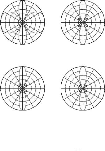
The matrix is ill-conditioned whenever cos ≈ 1, and is well-conditioned otherwise. In Figure 7.5, this quantity cos = fr%r is plotted as a function of %r for a fixed array size and different values of nr. The function fr · has the following properties:

fr%r is periodic with period nr/Lr = 1/r;

fr%r peaks at %r = 0; f0 = 1;

fr%r = 0 at %r = k/Lr k = 1 nr − 1.

The periodicity of fr · follows from the periodicity of the spatial signature er · . It has a main lobe of width 2/Lr centered around integer multiples of 1/r. All the other lobes have significantly lower peaks. This means that the signatures are close to being aligned and the channel matrix is ill conditioned

whenever


%r

m


1

(7.39)


r

Lr

for some integer m. Now, since %r ranges from −2 to 2, this condition reduces to

%r

1

(7.40)

Lr

whenever the antenna separation r ≤ 1/2.

303

7.2 Physical modeling of MIMO channels

Figure 7.5 The function |f( r )| plotted as a function of r for fixed Lr = 8 and different values of the number of receive antennas nr .

1


nr = 4


1


nr = 16


0.9


0.9


0.8


0.8


0.7


0.7


0.6


0.6


|f(Ωr)| 0.5


|f(Ωr)| 0.5


0.4


0.4


0.3


0.3


0.2


0.2


0.1


0.1


0

– 0.5

0

0.5

1

1.5

2

0

– 1 – 0.5

0

0.5

1

1.5

2

– 2 – 1.5 – 1

– 2 – 1.5


r


r


1

nr = 8


1

sinc function


0.9


0.9


0.8


0.8


0.7


0.7


0.6


0.6


|f(Ωr)| 0.5


|f(Ωr)| 0.5


0.4


0.4


0.3


0.3


0.2


0.2


0.1


0.1


0


0

0.5

1

1.5

2

0

– 1 – 0.5

0

0.5

1

1.5

2

– 2 – 1.5 – 1 – 0.5

– 2 – 1.5


r


r


Increasing the number of antennas for a fixed antenna length Lr does not substantially change the qualitative picture above. In fact, as nr → andr → 0,

fr%r → ejLr %r sincLr%r

(7.41)

and the dependency of fr · on nr vanishes. Equation (7.41) can be directly derived from (7.35), using the definition sincx = sinx / x (cf. (2.30)).

The parameter 1/Lr can be thought of as a measure of resolvability in the angular domain: if %r 1/Lr, then the signals from the two transmit antennas cannot be resolved by the receive antenna array and there is effectively only one degree of freedom. Packing more and more antenna elements in a given amount of space does not increase the angular resolvability of the receive antenna array; it is intrinsically limited by the length of the array.

A common pictorial representation of the angular resolvability of an antenna array is the (receive) beamforming pattern. If the signal arrives from a single direction 0, then the optimal receiver projects the received signal onto the vector er cos 0 ; recall that this is called the (receive) beamforming vector. A signal from any other direction is attenuated by a factor of

er cos 0 er cos = fr cos − cos 0

(7.42)

The beamforming pattern associated with the vector er cos is the polar plot

fr cos − cos 0

(7.43)

304

MIMO I: spatial multiplexing and channel modeling

Figure 7.6 Receive beamforming patterns aimed at 90 , with antenna array length Lr = 2 and different numbers of receive antennas nr . Note that the beamforming pattern is always symmetrical about the 0 − 180 axis, so lobes always appear in pairs. For nr = 4 6 32, the antenna separation r ≤ 1/2, and there is a single main lobe around 90 (together with its mirror image). For nr = 2,

r = 1 > 1/2 and there is an additional pair of main lobes.

Lr = 2, nr = 2


Lr = 2, nr = 4


90

1


90

1

60

120

60


120

0.8


0.8


150

0.6


150

0.6

30

0.4

30

0.4


0.2


0.2


180


0

180


0

210


330

210


330

240

300


240


300

270


270


Lr = 2, nr = 6


Lr = 2, nr = 32


90

1


90

1


120

60


120

0.8

60


0.8


150

0.6

30


0.6

30

0.4

150

0.4


0.2


0.2


180


0

180


0

210


330

210


330


240

300


240


300

270


270


(Figures 7.6 and 7.7). Two important points to note about the beamforming pattern:

• It has main lobes around 0 and also around any angle for which

cos = cos 0 mod

1


(7.44)

r

this follows from the periodicity of fr · . If the antenna separation r is less than 1/2, then there is only one main lobe at , together with its mirror image at − . If the separation is greater than 1/2, there can be several more pairs of main lobes (Figure 7.6).

The main lobe has a directional cosine width of 2/Lr; this is also called the beam width. The larger the array length Lr, the narrower the beam and the higher the angular resolution: the array filters out the signal from

all directions except for a narrow range around the direction of interest (Figure 7.7). Signals that arrive along paths with angular seperation larger than 1/Lr can be discriminated by focusing different beams at them.

There is a clear analogy between the roles of the antenna array size Lr and the bandwidth W in a wireless channel. The parameter 1/W measures the

305

7.2 Physical modeling of MIMO channels


Figure 7.7 Beamforming


Lr = 4, nr = 8


Lr = 8, nr = 16


patterns for different antenna


90

1


90

1


array lengths. (Left) Lr = 4 and

120


60


120


60


(right) Lr = 8. Antenna

150


0.5

30

150


0.5

30

separation is fixed at half the


carrier wavelength. The larger


the length of the array, the

180


0

180


0

narrower the beam.


210


330

210


330


240

270

300


240


300


270


resolvability of signals in the time domain: multipaths arriving at time separation much less than 1/W cannot be resolved by the receiver. The parameter 1/Lr measures the resolvability of signals in the angular domain: signals that arrive within an angle much less than 1/Lr cannot be resolved by the receiver. Just as over-sampling cannot increase the time-domain resolvability beyond 1/W , adding more antenna elements cannot increase the angulardomain resolvability beyond 1/Lr. This analogy will be exploited in the statistical modeling of MIMO fading channels and explained more precisely in Section 7.3.

Geographically separated receive antennas

Figure 7.8 Two geographically separated receive antennas each with line-of-sight from a transmit antenna array.

We have increased the number of degrees of freedom by placing the transmit antennas far apart and keeping the receive antennas close together, but we can achieve the same goal by placing the receive antennas far apart and keeping the transmit antennas close together (see Figure 7.8). The channel matrix is given by

h

H = h1 (7.45)

2

Rx antenna 1


.


.


Tx antenna

.

φt2


array


φt1


Rx antenna 2

306 MIMO I: spatial multiplexing and channel modeling

where


hi = ai exp

j2

d

i1

et %ti

(7.46)


c


and %ti is the directional cosine of departure of the path from the transmit antenna array to receive antenna i and di1 is the distance between transmit antenna 1 and receive antenna i. As long as

%t = %t2 − %t1 =0 mod

1


(7.47)

t

the two rows of H are linearly independent and the channel has rank 2, yielding 2 degrees of freedom. The output of the channel spans a two-dimensional space as we vary the transmitted signal at the transmit antenna array. In order to make H well-conditioned, the angular separation %t of the two receive antennas should be of the order of or larger than 1/Lt, where Lt = nt t is the length of the transmit antenna array, normalized to the carrier wavelength.

Analogous to the receive beamforming pattern, one can also define a transmit beamforming pattern. This measures the amount of energy dissipated in other directions when the transmitter attempts to focus its signal along a direction 0. The beam width is 2/Lt; the longer the antenna array, the sharper the transmitter can focus the energy along a desired direction and the better it can spatially multiplex information to the multiple receive antennas.

7.2.5 Line-of-sight plus one reflected path

Can we get a similar effect to that of the example in Section 7.2.4, without putting either the transmit antennas or the receive antennas far apart? Consider again the transmit and receive antenna arrays in that example, but now suppose in addition to a line-of-sight path there is another path reflected off a wall (see Figure 7.9(a)). Call the direct path, path 1 and the reflected path, path 2. Path i has an attenuation of ai, makes an angle of ti (%ti = cos ti) with the transmit antenna array and an angle of ri %ri = cos ri) with the receive antenna array. The channel H is given by the principle of superposition:

H = a1ber %r1 et %t1 + a2ber %r2 er %t2

(7.48)

where for i = 1 2,


aib = ai


exp −

j2 d i

(7.49)

ntnr


c

and d i is the distance between transmit antenna 1 and receive antenna 1 along path i. We see that as long as

%t1 =%t2 mod

1

(7.50)

t

307

7.2 Physical modeling of MIMO channels

Figure 7.9 (a) A MIMO channel with a direct path and a reflected path. (b) Channel is viewed as a concatenation of two channels H and H with intermediate (virtual) relays

A and B.


A


~

path 2


~


~


Tx antenna 1

φ

t2


~


Tx antenna


φt1


path 1


φr2


~


array


Rx antenna


~


φr1


B


array


(a)

Rx antenna 1


A


Tx antenna

.


H


H

.


Rx antenna

array


.


B


.


array


.


.


(b)

and

%r1 =%r2 mod

1


(7.51)

r

the matrix H is of rank 2. In order to make H well-conditioned, the angular separation %t of the two paths at the transmit array should be of the same order or larger than 1/Lt and the angular separation %r at the receive array should be of the same order as or larger than 1/Lr, where

%t

= cos t2 − cos t1

Lt

= nt t

(7.52)

and


%r

= cos r2 − cos r1

Lr

= nr r

(7.53)

To see clearly what the role of the multipath is, it is helpful to rewrite H as H = H H , where

H =

a1er

%r1

a2er%r2


H =

e %


(7.54)

et %t2


b


b


t

t1


H is a 2 by nt matrix while H is an nr by 2 matrix. One can interpret H as the matrix for the channel from the transmit antenna array to two imaginary receivers at point A and point B, as marked in Figure 7.9. Point A is the point of incidence of the reflected path on the wall; point B is along the line-of-sight path. Since points A and B are geographically widely separated, the matrix H has rank 2; its conditioning depends on the parameter Lt%t. Similarly,