Добавил:
Upload Опубликованный материал нарушает ваши авторские права? Сообщите нам.
Вуз: Предмет: Файл:

Fundamentals Of Wireless Communication

.pdf
Скачиваний:
87
Добавлен:
15.03.2015
Размер:
10.3 Mб
Скачать

288

Multiuser capacity and opportunistic communication

respectively. Show that superposition coding is strictly better than the orthogonal schemes, i.e., for every non-zero rate pair achieved by an orthogonal scheme, there is a superposition coding scheme which allows each user to strictly increase its rate.

Exercise 6.26 A reading exercise is to study [8], where the sufficiency of superposition encoding and decoding for the downlink AWGN channel is shown.

Exercise 6.27 Consider the two-user symmetric downlink fading channel with receiver CSI alone (cf. (6.50)). We have seen that the capacity region of the downlink channel does not depend on the correlation between the additive noise processes z1m and z2m (cf. Exercise 6.24(1)). Consider the following specific correlation: z1m z2m are 0 Km and independent in time m. To preserve the marginal variance, the diagonal entries of the covariance matrix Km must be N0 each. Let us denote the off-diagonal term by " m N0 (with " m ≤ 1). Suppose now we let the two users cooperate.

1. Show that by a careful choice of " m (as a function of h1m and h2m), cooperation is not gainful: that is, for any reliable rates R1 R2 in the downlink fading channel,


1

+


2


+

N0


R


R


log 1


h 2P


(6.92)


the same as can be achieved by a single user alone (cf. (6.51)). Here distribution of h is the symmetric stationary distribution of the fading processes hkm (for k = 1 2). Hint: You will find Exercise 6.24(3) useful.

2.Conclude that the capacity region of the symmetric downlink fading channel is that given by (6.92).

Exercise 6.28 Show that the proportional fair algorithm with an infinite time-scale window maximizes (among all scheduling algorithms) the sum of the logarithms of the throughputs of the users. This justifies (6.57). This result has been derived in the literature at several places, including [12].

Exercise 6.29 Consider the opportunistic beamforming scheme in conjunction with a proportional fair scheduler operating in a slow fading environment. A reading exercise is to study Theorem 1 of [137], which shows that the rate available to each user is approximately equal to the instantaneous rate when it is being transmit beamformed, scaled down by the number of users.

Exercise 6.30 In a cellular system, the multiuser diversity gain in the downlink is expressed through the maximum SINR (cf. (6.63))

SINR

max


= k

max

SINR

k =

P hk 2


(6.93)

J

gkj

2


=


N0 + P j=1


where we have denoted P by the average received power at a user. Let us denote the ratio P/N0 by SNR. Let us suppose that h1 hK are i.i.d. 0 1 random

variables, and gkj k = 1 K j = 1 J are i.i.d. 0 0 2 random variables independent of h. (A factor of 0.2 is used to model the average scenario of the mobile

user being closer to the base-station it is communicating with as opposed to all the other base-stations it is hearing interference from, cf. Section 4.2.3.)

289

6.9 Exercises


1. Show using the limit theorem in Exercise 6.21 that


SINRmax

→ 1

as K →

(6.94)


xK


where xK satisfies the non-linear equation:


1 +

xK

J

xK


= K exp


(6.95)


5


SNR


2.Plot xK for K = 1 16 for different values of SNR (ranging from 0 dB to 20 dB).

Can you intuitively justify the observation from the plot that xK increases with increasing SNR values? Hint: The probability that hk 2 is less than or equal to a small positive number is approximately equal to itself, while the probability thathk 2 is larger than a large number 1/ is exp −1/ . Thus the likely way SINR becomes large is by the denominator being small as opposed to the numerator

becoming large.

3.Show using part (1), or directly, that at small values of SNR the mean of the

effective SINR grows like log K. You can also see this directly from (6.93): at small values of SNR, the effective SINR is simply the maximum of K Rayleigh distributed random variables and from Exercise 6.21(2) we know that the mean value grows like log K.

4.At very high values of SNR, we can approximate exp −xK /SNR in (6.95) by 1. With this approximation, show, using part (1), that the scaling xK is approximately like K1/J . This is a faster growth rate than the one at low SNR.

5.In a cellular system, typically the value of P is chosen such that the background noise N0 and the interference term are of the same order. This makes sense for a

system where there is no scheduling of users: since the system is interference plus noise limited, there is no point in making one of them (interference or background noise) much smaller than the other. In our notation here, this means that SNR is approximately 0 dB. From the calculations of this exercise what design setting of P can you infer for a system using the multiuser diversity harnessing scheduler? Thus, conventional transmit power settings will have to be revisited in this new system point of view.

Exercise 6.31 (Interaction between space-time codes and multiuser diversity scheduling) A design is proposed for the downlink IS-856 using dual transmit antennas at the base-station. It employs the Alamouti scheme when transmitting to a single user and among the users schedules the user with the best effective instantaneous SNR under the Alamouti scheme. We would like to compare the performance gain, if any, of using this scheme as opposed to using just a single transmit antenna and scheduling to the user with the best instantaneous SNR. Assume independent Rayleigh fading across the transmit antennas.

1.Plot the distribution of the instantaneous effective SNR under the Alamouti scheme, and compare that to the distribution of the SNR for a single antenna.

2.Suppose there is only a single user (i.e., K = 1). From your plot in part (1), do you think the dual transmit antennas provide any gain? Justify your answer. Hint: Use Jensen’s inequality.

3.How about when K > 1? Plot the achievable throughput under both schemes at average SNR = 0 dB and for different values of K.

4.Is the proposed way of using dual transmit antennas smart?

C H A P T E R

7MIMO I: spatial multiplexing and channel modeling

In this book, we have seen several different uses of multiple antennas in wireless communication. In Chapter 3, multiple antennas were used to provide diversity gain and increase the reliability of wireless links. Both receive and transmit diversity were considered. Moreover, receive antennas can also provide a power gain. In Chapter 5, we saw that with channel knowledge at the transmitter, multiple transmit antennas can also provide a power gain via transmit beamforming. In Chapter 6, multiple transmit antennas were used to induce channel variations, which can then be exploited by opportunistic communication techniques. The scheme can be interpreted as opportunistic beamforming and provides a power gain as well.

In this and the next few chapters, we will study a new way to use multiple antennas. We will see that under suitable channel fading conditions, having both multiple transmit and multiple receive antennas (i.e., a MIMO channel) provides an additional spatial dimension for communication and yields a degree-of- freedom gain. These additional degrees of freedom can be exploited by spatially multiplexing several data streams onto the MIMO channel, and lead to an increase in the capacity: the capacity of such a MIMO channel with n transmit and receive antennas is proportional to n.

Historically, it has been known for a while that a multiple access system with multiple antennas at the base-station allows several users to simultaneously communicate with the base-station. The multiple antennas allow spatial separation of the signals from the different users. It was observed in the mid 1990s that a similar effect can occur for a point-to-point channel with multiple transmit and receive antennas, i.e., even when the transmit antennas are not geographically far apart. This holds provided that the scattering environment is rich enough to allow the receive antennas to separate out the signals from the different transmit antennas. We have already seen how channel fading can be exploited by opportunistic communication techniques. Here, we see yet another example where channel fading is beneficial to communication.

It is insightful to compare and contrast the nature of the performance gains offered by opportunistic communication and by MIMO techniques.

290

291 7.1 Multiplexing capability of deterministic MIMO channels

Opportunistic communication techniques primarily provide a power gain. This power gain is very significant in the low SNR regime where systems are power-limited but less so in the high SNR regime where they are bandwidthlimited. As we will see, MIMO techniques can provide both a power gain and a degree-of-freedom gain. Thus, MIMO techniques become the primary tool to increase capacity significantly in the high SNR regime.

MIMO communication is a rich subject, and its study will span the remaining chapters of the book. The focus of the present chapter is to investigate the properties of the physical environment which enable spatial multiplexing and show how these properties can be succinctly captured in a statistical MIMO channel model. We proceed as follows. Through a capacity analysis, we first identify key parameters that determine the multiplexing capability of a deterministic MIMO channel. We then go through a sequence of physical MIMO channels to assess their spatial multiplexing capabilities. Building on the insights from these examples, we argue that it is most natural to model the MIMO channel in the angular domain and discuss a statistical model based on that approach. Our approach here parallels that in Chapter 2, where we started with a few idealized examples of multipath wireless channels to gain insights into the underlying physical phenomena, and proceeded to statistical fading models, which are more appropriate for the design and performance analysis of communication schemes. We will in fact see a lot of parallelism in the specific channel modeling technique as well.

Our focus throughout is on flat fading MIMO channels. The extensions to frequency-selective MIMO channels are straightforward and are developed in the exercises.

7.1 Multiplexing capability of deterministic MIMO channels

A narrowband time-invariant wireless channel with nt transmit and nr receive antennas is described by an nr by nt deterministic matrix H. What are the key properties of H that determine how much spatial multiplexing it can support? We answer this question by looking at the capacity of the channel.

7.1.1 Capacity via singular value decomposition

The time-invariant channel is described by

y = Hx + w

(7.1)

where x nt , y nr and w 0 N0Inr denote the transmitted signal, received signal and white Gaussian noise respectively at a symbol time (the time index is dropped for simplicity). The channel matrix H nr ×nt

292

MIMO I: spatial multiplexing and channel modeling

is deterministic and assumed to be constant at all times and known to both the transmitter and the receiver. Here, hij is the channel gain from transmit antenna j to receive antenna i. There is a total power constraint, P, on the signals from the transmit antennas.

This is a vector Gaussian channel. The capacity can be computed by decomposing the vector channel into a set of parallel, independent scalar Gaussian sub-channels. From basic linear algebra, every linear transformation can be represented as a composition of three operations: a rotation operation, a scaling operation, and another rotation operation. In the notation of matrices, the matrix H has a singular value decomposition (SVD):

H = U V

(7.2)

where U nr ×nr and V nt ×nt are (rotation) unitary matrices1

and

nr ×nt is a rectangular matrix whose diagonal elements are non-negative real numbers and whose off-diagonal elements are zero.2 The diagonal elements

1 2 ≥ · · · ≥ nmin are the ordered singular values of the matrix H, where nmin = minnt nr . Since

HH = U tU

(7.3)

the squared singular values 2i are the eigenvalues of the matrix HH and also of H H. Note that there are nmin singular values. We can rewrite the SVD as


nmin


H =


iuivi

(7.4)

i=1

i.e., the sum of rank-one matrices iuivi . It can be seen that the rank of H is precisely the number of non-zero singular values.

If we define

= V x

(7.5)

= U y

(7.6)

= U w

(7.7)

then we can rewrite the channel (7.1) as

y˜ = x˜ + w˜

(7.8)

2

Recall that a unitary matrix U satisfies U U

=

UU

=

I.

1


We will call this matrix diagonal even though it may not be square.

293

Figure 7.1 Converting the MIMO channel into a parallel channel through the SVD.

7.1 Multiplexing capability of deterministic MIMO channels


λ1

w

1


×


+


.


x


.


y


~

x


V


V*


λnmin .

wnmin

U


U*


y


×


+


Pre-

processing


Channel


Post-processing


where w˜ 0 N0Inr has the same distribution as w (cf. (A.22) in Appendix A), and x˜ 2 = x 2. Thus, the energy is preserved and we have an equivalent representation as a parallel Gaussian channel:

i = ii + w˜ i

i = 1 2 nmin

(7.9)

The equivalence is summarized in Figure 7.1.

The SVD decomposition can be interpreted as two coordinate transformations: it says that if the input is expressed in terms of a coordinate system defined by the columns of V and the output is expressed in terms of a coordinate system defined by the columns of U, then the input/output relationship is very simple. Equation (7.8) is a representation of the original channel (7.1) with the input and output expressed in terms of these new coordinates.

We have already seen examples of Gaussian parallel channels in Chapter 5, when we talked about capacities of time-invariant frequency-selective channels and about time-varying fading channels with full CSI. The time-invariant MIMO channel is yet another example. Here, the spatial dimension plays the same role as the time and frequency dimensions in those other problems. The capacity is by now familiar:


P 2


nmin


C = i=1 log

1 +

i


i

bits/s/Hz


(7.10)


N

0

where P P are the waterfilling power allocations:


1

nmin


= −

N0

+


Pi


(7.11)


i2


with chosen to satisfy the total power constraint i Pi = P. Each i corresponds to an eigenmode of the channel (also called an eigenchannel). Each non-zero eigenchannel can support a data stream; thus, the MIMO channel can support the spatial multiplexing of multiple streams. Figure 7.2 pictorially depicts the SVD-based architecture for reliable communication.

294

MIMO I: spatial multiplexing and channel modeling


~


~

[m]}


AWGN


{x1[m]}


{y1

Decoder


coder


.


n min

.


{w[m]}


.


.


information


.


.


streams


~


~


AWGN

{xnmin[m]}

V


H


+


U*

{ynmin[m]}

Decoder


coder


{0}


.


.


.

{0}


Figure 7.2 The SVD architecture for MIMO communication.

There is a clear analogy between this architecture and the OFDM system introduced in Chapter 3. In both cases, a transformation is applied to convert a matrix channel into a set of parallel independent sub-channels. In the OFDM setting, the matrix channel is given by the circulant matrix C in (3.139), defined by the ISI channel together with the cyclic prefix added onto the input symbols. In fact, the decomposition C = Q−1 Q in (3.143) is the SVD decomposition of a circulant matrix C, with U = Q−1 and V = Q. The important difference between the ISI channel and the MIMO channel is that, for the former, the U and V matrices (DFTs) do not depend on the specific realization of the ISI channel, while for the latter, they do depend on the specific realization of the MIMO channel.

7.1.2 Rank and condition number

What are the key parameters that determine performance? It is simpler to focus separately on the high and the low SNR regimes. At high SNR, the water level is deep and the policy of allocating equal amounts of power on the non-zero eigenmodes is asymptotically optimal (cf. Figure 5.24(a)):

k

P 2


k

2

bits/s/Hz (7.12)

C ≈ log 1 +

i

≈ k log SNR + log

i

kN0

k

i=1


i=1


where k is the number of non-zero 2i , i.e., the rank of H, and SNR = P/N0.

The parameter k is the number of spatial degrees of freedom per second per hertz. It represents the dimension of the transmitted signal as modified by the MIMO channel, i.e., the dimension of the image of H. This is equal to the rank of the matrix H and with full rank, we see that a MIMO channel provides nmin spatial degrees of freedom.

295

7.2 Physical modeling of MIMO channels

The rank is a first-order but crude measure of the capacity of the channel. To get a more refined picture, one needs to look at the non-zero singular values themselves. By Jensen’s inequality,

k i=1 log

1 + kN0

i2


≤ log

1 + kN0

k i=1

i2


(7.13)

1

k


P


P

1

k


Now,

k


= Tr HH =

hij 2


i2


(7.14)

i=1


i j


which can be interpreted as the total power gain of the matrix channel if one spreads the energy equally between all the transmit antennas. Then, the above result says that among the channels with the same total power gain, the one that has the highest capacity is the one with all the singular values equal. More generally, the less spread out the singular values, the larger the capacity in the high SNR regime. In numerical analysis, maxi i/ mini i is defined to be the condition number of the matrix H. The matrix is said to be well-conditioned if the condition number is close to 1. From the above result, an important conclusion is:

Well-conditioned channel matrices facilitate communication in the high

SNR regime.

At low SNR, the optimal policy is to allocate power only to the strongest eigenmode (the bottom of the vessel to waterfill, cf. Figure 5.24(b)). The resulting capacity is

P

maxi

i2 log2 e bits/s/Hz


C ≈ N0

(7.15)

The MIMO channel provides a power gain of maxi 2i . In this regime, the rank or condition number of the channel matrix is less relevant. What matters is how much energy gets transferred from the transmitter to the receiver.

7.2 Physical modeling of MIMO channels

In this section, we would like to gain some insight on how the spatial multiplexing capability of MIMO channels depends on the physical environment. We do so by looking at a sequence of idealized examples and analyzing the

296 MIMO I: spatial multiplexing and channel modeling

rank and conditioning of their channel matrices. These deterministic examples will also suggest a natural approach to statistical modeling of MIMO channels, which we discuss in Section 7.3. To be concrete, we restrict ourselves to uniform linear antenna arrays, where the antennas are evenly spaced on a straight line. The details of the analysis depend on the specific array structure but the concepts we want to convey do not.

7.2.1 Line-of-sight SIMO channel

Figure 7.3 (a) Line-of-sight channel with single transmit antenna and multiple receive antennas. The signals from the transmit antenna arrive almost in parallel at the receiving antennas. (b) Line-of-sight channel with multiple transmit antennas and single receive antenna.

The simplest SIMO channel has a single line-of-sight (Figure 7.3(a)). Here, there is only free space without any reflectors or scatterers, and only a direct signal path between each antenna pair. The antenna separation is r c, where c is the carrier wavelength and r is the normalized receive antenna separation, normalized to the unit of the carrier wavelength. The dimension of the antenna array is much smaller than the distance between the transmitter and the receiver.

The continuous-time impulse response hi between the transmit antenna and the ith receive antenna is given by

hi = a − di/c

d

(a)

. . .

Tx antenna i

. . . d

tλc φ

(i −1)∆tλccosφ

(b)

i = 1 nr

(7.16)


.


.


.

(i −1)∆rλccosφ

Rx antenna i

.

.

.

rλc

φ

297

7.2 Physical modeling of MIMO channels

where di is the distance between the transmit antenna and ith receive antenna, c is the speed of light and a is the attenuation of the path, which we assume to be the same for all antenna pairs. Assuming di/c 1/W , where W is the transmission bandwidth, the baseband channel gain is given by (2.34) and (2.27):

hi = a exp −

j2f

d

i


= a exp −

d

i


c


j2

(7.17)

c


c


where fc is the carrier frequency. The SIMO channel can be written as

y = hx + w

(7.18)

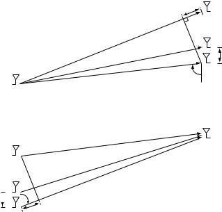
where x is the transmitted symbol, w 0 N0I is the noise and y is the received vector. The vector of channel gains h = h1 hnr t is sometimes called the signal direction or the spatial signature induced on the receive antenna array by the transmitted signal.

Since the distance between the transmitter and the receiver is much larger than the size of the receive antenna array, the paths from the transmit antenna to each of the receive antennas are, to a first-order, parallel and

di ≈ d + i − 1 r c cos i = 1 nr

(7.19)

where d is the distance from the transmit antenna to the first receive antenna and is the angle of incidence of the line-of-sight onto the receive antenna array. (You are asked to verify this in Exercise 7.1.) The quantity i−1 r c cos is the displacement of receive antenna i from receive antenna 1 in the direction of the line-of-sight. The quantity

% = cos

is often called the directional cosine with respect to the receive antenna array. The spatial signature h = h1 hnr t is therefore given by


1


exp −j2 r%


=


c


h

a exp j2d


(7.20)


exp −j2 2 r%


exp j2nr

1 r%