

Fundamentals Of Wireless Communication
.pdf328 |
MIMO I: spatial multiplexing and channel modeling |
distributed and circular symmetric complex Gaussian. Since the matrix H m and its angular domain representation Ha m are related by
Ha m = Ur H m Ut |
(7.80) |
and Ur and Ut are fixed unitary matrices, this means that Ha should have the same i.i.d. Gaussian distribution as H. Thus, using the modeling approach described here, we can see clearly the physical basis of the i.i.d Rayleigh fading model, in terms of both the multipath environment and the antenna arrays. There should be a significant number of multipaths in each of the resolvable angular bins, and the energy should be equally spread out across these bins. This is the socalled richly scattered environment. If there are very few or no paths in some of the angular directions, then the entries in H will be correlated. Moreover, the antennas should be either critically or sparsely spaced. If the antennas are densely spaced, then some entries of Ha are approximately zero and the entries in H itself are highly correlated. However, by a simple transformation, the channel can be reduced to an equivalent channel with fewer antennas which are critically spaced.
Compared to the critically spaced case, having sparser spacing makes it easier for the channel matrix to satisfy the i.i.d. Rayleigh assumption. This is because each bin now spans more distinct angular windows and thus contains more paths, from multiple transmit and receive directions. This substantiates the intuition that putting the antennas further apart makes the entries of H less dependent. On the other, if the physical environment already provides scattering in all directions, then having critical spacing of the antennas is enough to satisfy the i.i.d. Rayleigh assumption.
Due to the analytical tractability, we will use the i.i.d. Rayleigh fading model quite often to evaluate performance of MIMO communication schemes, but it is important to keep in mind the assumptions on both the physical environment and the antenna arrays for the model to be valid.
Chapter 7 The main plot
The angular domain provides a natural representation of the MIMO channel, highlighting the interaction between the antenna arrays and the physical environment.
The angular resolution of a linear antenna array is dictated by its length: an array of length L provides a resolution of 1/L. Critical spacing of antenna
elements at half the carrier wavelength captures the full angular resolution of 1/L. Sparser spacing reduces the angular resolution due to aliasing. Denser spacing does not increase the resolution beyond 1/L.
Transmit and receive antenna arrays of length Lt and Lr partition the angular domain into 2Lt × 2Lr bins of unresolvable multipaths. Paths that fall within the same bin are aggregated to form one entry of the angular channel matrix Ha.

329 |
7.4 Bibliographical notes |
A statistical model of Ha is obtained by assuming independent Gaussian distributed entries, of possibly different variances. Angular bins that contain no paths correspond to zero entries.
The number of degrees of freedom in the MIMO channel is the minimum of the number of non-zero rows and the number of non-zero columns of Ha. The amount of diversity is the number of non-zero entries.
In a clustered-response model, the number of degrees of freedom is approximately:
min Lt%t total Lr%r total |
(7.81) |
The multiplexing capability of a MIMO channel increases with the angu-
lar spreads %t total %r total of the scatterers/reflectors as well as with the antenna array lengths. This number of degrees of freedom can be
achieved when the antennas are critically spaced at half the wavelength or closer. With a maximum angular spread of 2, the number of degrees of freedom is
min 2Lt 2Lr
and this equals
min nt nr
when the antennas are critically spaced.
The i.i.d. Rayleigh fading model is reasonable in a richly scattering environment where the angular bins are fully populated with paths and there is roughly equal amount of energy in each bin. The antenna elements should be critically or sparsely spaced.
7.4 Bibliographical notes
The angular domain approach to MIMO channel modeling is based on works by Sayeed [105] and Poon et al. [90, 92]. [105] considered an array of discrete antenna elements, while [90, 92] considered a continuum of antenna elements to emphasize that spatial multiplexability is limited not by the number of antenna elements but by the size of the antenna array. We considered only linear arrays in this chapter, but [90] also treated other antenna array configurations such as circular rings and spherical surfaces. The degree-of-freedom formula (7.78) is derived in [90] for the clustered response model.
Other related approaches to MIMO channel modeling are by Raleigh and Cioffi [97], by Gesbert et al. [47] and by Shiu et al. [111]. The latter work used a Clarke-like model but with two rings of scatterers, one around the transmitter and one around the receiver, to derive the MIMO channel statistics.

330 |
MIMO I: spatial multiplexing and channel modeling |
7.5 Exercises
Exercise 7.1
1.For the SIMO channel with uniform linear array in Section 7.2.1, give an exact expression for the distance between the transmit antenna and the ith receive antenna. Make precise in what sense is (7.19) an approximation.
2.Repeat the analysis for the approximation (7.27) in the MIMO case.
Exercise 7.2 Verify that the unit vector er%r , defined in (7.21), is periodic with period r and within one period never repeats itself.
Exercise 7.3 Verify (7.35).
Exercise 7.4 In an earlier work on MIMO communication [97], it is stated that the number of degrees of freedom in a MIMO channel with nt transmit, nr receive antennas and K multipaths is given by
min nt nr K |
(7.82) |
and this is the key parameter that determines the multiplexing capability of the channel. What are the problems with this statement?
Exercise 7.5 In this question we study the role of antenna spacing in the angular representation of the MIMO channel.
1.Consider the critically spaced antenna array in Figure 7.21; there are six bins, each one corresponding to a specific physical angular window. All of these angular windows have the same width as measured in solid angle. Compute the angular window width in radians for each of the bins l, with l = 0 5. Argue that the width in radians increases as we move from the line perpendicular to the antenna array to one that is parallel to it.
2.Now consider the sparsely spaced antenna arrays in Figure 7.22. Justify the depicted
mapping from the angular windows to the bins l and evaluate the angular window width in radians for each of the bins l (for l = 0 1 nt − 1). (The angular window width of a bin l is the sum of the widths of all the angular windows that correspond to the bin l.)
3.Justify the depiction of the mapping from angular windows to the bins l in the densely spaced antenna array of Figure 7.23. Also evaluate the angular width of
each bin in radians.
Exercise 7.6 The non-zero entries of the angular matrix Ha are distributed as independent complex Gaussian random variables. Show that with probability 1, the rank of the matrix is given by the formula (7.74).
Exercise 7.7 In Chapter 2, we introduced Clarke’s flat fading model, where both the transmitter and the receiver have a single antenna. Suppose now that the receiver has nr antennas, each spaced by half a wavelength. The transmitter still has one antenna (a SIMO channel). At time m
ym = hm x m + wm |
(7.83) |
where ym hm are the nr -dimensional received vector and receive spatial signature (induced by the channel), respectively.
331 |
7.5 Exercises |
1.Consider first the case when the receiver is stationary. Compute approximately the joint statistics of the coefficients of h in the angular domain.
2.Now suppose the receiver is moving at a speed v. Compute the Doppler spread and the Doppler spectrum of each of the angular domain coefficients of the channel.
3.What happens to the Doppler spread as nr → ? What can you say about the difficulty of estimating and tracking the process hm as n grows? Easier, harder,
or the same? Explain.
Exercise 7.8 [90] Consider a circular array of radius R normalized by the carrier wavelength with n elements uniformly spaced.
1. |
Compute the spatial signature in the direction . |
2. |
Find the angle, f1 2 , between the two spatial signatures in the direction 1 |
|
and 2. |
3. |
Does f1 2 only depend on the difference 1 − 2? If not, explain why. |
4. |
Plot f1 0 for R = 2 and different values of n, from n equal to R/2", R", |
|
2R", to 4R". Observe the plot and describe your deductions. |
5. |
Deduce the angular resolution. |
6. |
Linear arrays of length L have a resolution of 1/L along the cos -domain, that |
|
is, they have non-uniform resolution along the -domain. Can you design a linear |
|
array with uniform resolution along the -domain? |
Exercise 7.9 (Spatial sampling) Consider a MIMO system with Lt = Lr = 2 in a channel with M = 10 multipaths. The ith multipath makes an angle of i with the transmit array and an angle of i with the receive array where = /M.
1.Assuming there are nt transmit and nr receive antennas, compute the channel matrix.
2.Compute the channel eigenvalues for nt = nr varying from 4 to 8.
3.Describe the distribution of the eigenvalues and contrast it with the binning interpretation in Section 7.3.4.
Exercise 7.10 In this exercise, we study the angular domain representation of frequency-selective MIMO channels.
1.Starting with the representation of the frequency-selective MIMO channel in time (cf. (8.112)) describe how you would arrive at the angular domain equivalent (cf. (7.69)):
|
L−1 |
|
yam = |
|
|
Hamxam − + wam |
(7.84) |
=0
2.Consider the equivalent (except for the overhead in using the cyclic prefix) parallel MIMO channel as in (8.113).
(a)Discuss the role played by the density of the scatterers and the delay spread in
˜
the physical environment in arriving at an appropriate statistical model for Hn at the different OFDM tones n.
˜
(b) Argue that the (marginal) distribution of the MIMO channel Hn is the same for each of the tones n = 0 N − 1.
Exercise 7.11 A MIMO channel has a single cluster with the directional cosine ranges as &t = &r = 0 1 . Compute the number of degrees of freedom of an n × n channel as a function of the antenna separation t = r = .


334 |
MIMO II: capacity and multiplexing architectures |
|
|
|
|
|
|
|
|
|||||
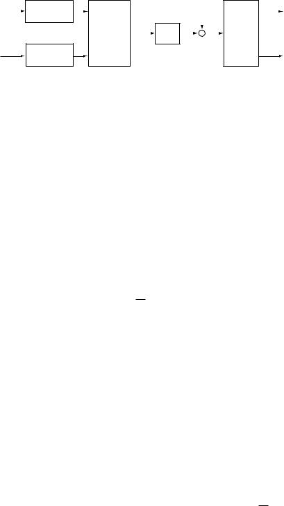
Figure 8.1 The V-BLAST |
P1 |
AWGN coder |
|
|
|
|
|
|
w[m] |
|
|
|||
architecture for communicating |
|
|
|
|
|
|
|
|
||||||
|
rate R1 |
|
|
|
|
|
|
|
|
|
|
|
|
|
|
|
|
|
|
|
|
|
|
|
|
|
|
||
over the MIMO channel. |
|
|
|
|
|
|
|
|
|
|
|
|
· |
|
|
|
|
|
|
|
|
|
|
|
y[m] |
|
|||
|
|
· |
|
|
x[m] |
|
|
|
|
Joint |
· |
|||
|
|
|
|
|
|
|
|
|
|
|
|
· |
||
|
|
· |
|
Q |
|
|
H[m] |
|
+ |
|
|
|
· |
|
|
|
|
|
|
|
|||||||||
|
|
· |
|
|
|
|
|
|
|
|
|
|
decoder |
· |
|
|
· |
|
|
|
|
|
|
|
|
|
|
· |
|
|
|
|
|
|
|
|
|
|
|
|
|
|
|
· |
|
Pnt |
AWGN coder |
|
|
|
|
|
|
|
|
|
|
|
· |
|
|
|
|
|
|
|
|
|
|
|
|
|
||
rate Rnt
coordinate system given by a unitary matrix Q, not necessarily dependent on the channel matrix H. This is the V-BLAST architecture. The data streams are decoded jointly. The kth data stream is allocated a power Pk (such that the sum of the powers, P1 + · · · + Pnt , is equal to P, the total transmit power constraint) and is encoded using a capacity-achieving Gaussian code with rate Rk. The total rate is R = nk=t 1 Rk.
As special cases:
•If Q = V and the powers are given by the waterfilling allocations, then we have the capacity-achieving architecture in Figure 7.2.
•If Q = Inr , then independent data streams are sent on the different transmit antennas.
Using a sphere-packing argument analogous to the ones used in Chapter 5, we will argue an upper bound on the highest reliable rate of communication:
1 |
HKxH bits/s/Hz |
|
R < log det Inr + N0 |
(8.2) |
Here Kx is the covariance matrix of the transmitted signal x and is a function of the multiplexing coordinate system and the power allocations:
Kx = Q diag P1 Pnt Q |
(8.3) |
Considering communication over a block of time symbols of length N , the received vector, of length nrN , lies with high probability in an ellipsoid of volume proportional to
det N0Inr + HKxH N |
(8.4) |
This formula is a direct generalization of the corresponding volume for-
mula (5.50) for the parallel channel, and is justified in Exercise 8.2. Since
√
we have to allow for non-overlapping noise spheres (of radius N0 and, hence, volume proportional to N0nr N ) around each codeword to ensure reliable
335 |
8.2 Fast fading MIMO channel |
communication, the maximum number of codewords that can be packed is the ratio
detN0Inr + HKxH N |
|
(8.5) |
|
N0nr N |
|||
|
|
We can now conclude the upper bound on the rate of reliable communication in (8.2).
Is this upper bound actually achievable by the V-BLAST architecture? Observe that independent data streams are multiplexed in V-BLAST; perhaps coding across the streams is required to achieve the upper bound (8.2)? To get some insight on this question, consider the special case of a MISO channel (nr = 1) and set Q = Int in the architecture, i.e., independent streams on each of the transmit antennas. This is precisely an uplink channel, as considered in Section 6.1, drawing an analogy between the transmit antennas and the users. We know from the development there that the sum capacity of this uplink channel is
|
|
+ |
kn=t |
N0 |
|
|
log |
1 |
|
1 hk 2Pk |
|
(8.6) |
This is precisely the upper bound (8.2) in this special case. Thus, the V-BLAST architecture, with independent data streams, is sufficient to achieve the upper bound (8.2). In the general case, an analogy can be drawn between the V-BLAST architecture and an uplink channel with nr receive antennas and channel matrix HQ; just as in the single receive antenna case, the upper bound (8.2) is the sum capacity of this uplink channel and therefore achievable using the V-BLAST architecture. This uplink channel is considered in greater detail in Chapter 10 and its information theoretic analysis is in Appendix B.9.
8.2 Fast fading MIMO channel
The fast fading MIMO channel is
ym = Hmxm + wm m = 1 2 |
(8.7) |
where Hm is a random fading process. To properly define a notion of capacity (achieved by averaging of the channel fading over time), we make the technical assumption (as in the earlier chapters) that Hm is a stationary and ergodic process. As a normalization, let us suppose that hij 2 = 1. As in our earlier study, we consider coherent communication: the receiver tracks the channel fading process exactly. We first start with the situation when the transmitter has only a statistical characterization of the fading channel. Finally, we look at the case when the transmitter also perfectly tracks the fading

336 MIMO II: capacity and multiplexing architectures
channel (full CSI); this situation is very similar to that of the time-invariant MIMO channel.
8.2.1 Capacity with CSI at receiver
Consider using the V-BLAST architecture (Figure 8.1) with a channelindependent multiplexing coordinate system Q and power allocations P1 Pnt . The covariance matrix of the transmit signal is Kx and is not dependent on the channel realization. The rate achieved in a given channel state H is
1 |
HKxH |
|
log det Inr + N0 |
(8.8) |
As usual, by coding over many coherence time intervals of the channel, a long-term rate of reliable communication equal to
H log det Inr |
+ N0 |
HKxH |
(8.9) |
|
1 |
|
|
is achieved. We can now choose the covariance Kx as a function of the channel statistics to achieve a reliable communication rate of
C = Kx Tr Kx ≤P |
|
nr |
+ N0 |
x |
|
|
|
max |
log det I |
|
1 |
HK |
H |
|
(8.10) |
|
|
Here the trace constraint corresponds to the total transmit power constraint. This is indeed the capacity of the fast fading MIMO channel (a formal justification is in Appendix B.7.2). We emphasize that the input covariance is chosen to match the channel statistics rather than the channel realization, since the latter is not known at the transmitter.
The optimal Kx in (8.10) obviously depends on the stationary distribution of the channel process Hm. For example, if there are only a few dominant paths (no more than one in each of the angular bins) that are not timevarying, then we can view H as being deterministic. In this case, we know from Section 7.1.1 that the optimal coordinate system to multiplex the data streams is in the eigen-directions of H H and, further, to allocate powers in a waterfilling manner across the eigenmodes of H.
Let us now consider the other extreme: there are many paths (of approximately equal energy) in each of the angular bins. Some insight can be obtained by looking at the angular representation (cf. (7.80)): Ha = Ur HUt. The key advantage of this viewpoint is in statistical modeling: the entries of Ha are generated by different physical paths and can be modeled as being statistically independent (cf. Section 7.3.5). Here we are interested in the case when the entries of Ha have zero mean (no single dominant path in any of the angular

337 |
8.2 Fast fading MIMO channel |
windows). Due to independence, it seems reasonable to separately send information in each of the transmit angular windows, with powers corresponding to the strength of the paths in the angular windows. That is, the multiplexing is done in the coordinate system given by Ut (so Q = Ut in (8.3)). The covariance matrix now has the form
Kx = Ut Ut |
(8.11) |
where is a diagonal matrix with non-negative entries, representing the powers transmitted in the angular windows, so that the sum of the entries is equal to P. This is shown formally in Exercise 8.3, where we see that this observation holds even if the entries of Ha are only uncorrelated.
If there is additional symmetry among the transmit antennas, such as when the elements of Ha are i.i.d. 0 1 (the i.i.d. Rayleigh fading model), then one can further show that equal powers are allocated to each transmit angular window (see Exercises 8.4 and 8.6) and thus, in this case, the optimal covariance matrix is simply
P |
Int |
|
Kx = nt |
(8.12) |
More generally, the optimal powers (i.e., the diagonal entries of ) are chosen to be the solution to the maximization problem (substituting the angular
representation H |
= |
r |
|
t |
|
|
|
|
|
|
|
|
|
|
|
|
|
|
U |
HaU and (8.11) in (8.10)): |
|
|
|
|
|
||||||||
C = Tr ≤P |
|
|
nr |
+ N0 |
r |
|
|
|
|
r |
||||||
|
|
|
max |
log det |
I |
|
1 |
U |
Ha |
|
Ha U |
(8.13) |
||||
|
|
|
|
|
1 |
|
||||||||||
= |
|
max |
|
I |
|
|
Ha |
|
Ha |
|
||||||
|
|
|
|
|
|
|
||||||||||
Tr ≤P |
log det |
nr |
+ N0 |
|
|
|
|
|
|
(8.14) |
||||||
With equal powers (i.e., the optimal is equal to P/nt Int , the resulting capacity is
C = log det Inr |
+ nt |
HH |
(8.15) |
|
SNR |
|
|
|
|
|
|
where SNR = P/N0 is the common SNR at each receive antenna.
If 1 ≥ 2 ≥ · · · ≥ nmin are the (random) ordered singular values of H, then we can rewrite (8.15) as
|
|
|
|
SNR |
|
|
|
|
nmin |
|
|
|
|
|
|
C = i=1 |
log |
1 + |
|
i2 |
|
||
nt |
(8.16) |
||||||
= i=1 |
log |
1 + nt |
i2 |
|
|||
|
|
|
|
SNR |
|
|
|
nmin |
|
|
|
|
|
|
|