348 MIMO II: capacity and multiplexing architectures
Thus a power gain of a factor of nt is achieved by transmit beamforming. With dual transmit antennas, this is a gain of 3 dB.
At low SNR, there is a further gain from transmitter CSI due to dynamic allocation of power across the eigenmodes: at any given time, more power is given to stronger eigenmodes. This gain is of the same nature as the one from opportunistic communication discussed in Chapter 6.
What happens in the large antenna array regime? Applying the random matrix
result of Marcenko˘ and Pastur from Section 8.2.2, we conclude that the random
√ √
singular values i m / n of the channel matrix H m / n converge to the same deterministic limiting distribution f across all times m. This means that in the waterfilling strategy, there is no dynamic power allocation over time, only over space. This is sometimes known as a channel hardening effect.
Summary 8.1 Performance gains in a MIMO channel
The capacity of an nt × nr i.i.d. Rayleigh fading MIMO channel H with
receiver CSI is
+ nt
HH
Cnn SNR = log det Inr
(8.41)
SNR
At high SNR, the capacity is approximately equal (up to an additive constant) to nmin log SNR bits/s/Hz.
At low SNR, the capacity is approximately equal to nr SNR log2 e bits/s/Hz, so only a receive beamforming gain is realized.
With nt = nr = n, the capacity can be approximated by nc SNR where c SNR is the constant in (8.26).
Conclusion: In an n × n MIMO channel, the capacity increases linearly with n over the entire SNR range.
With channel knowledge at the transmitter, an additional nt/nr-fold transmit beamforming gain can be realized with an additional power gain from temporal–spatial waterfilling at low SNR.
8.3 Receiver architectures
The transceiver architecture of Figure 8.1 achieves the capacity of the fast fading MIMO channel with receiver CSI. The capacity is achieved by joint ML decoding of the data streams at the receiver, but the complexity grows exponentially with the number of data streams. Simpler decoding rules that provide soft information to feed to the decoders of the individual data streams is an active area of research; some of the approaches are reviewed
349 8.3 Receiver architectures
in Exercise 8.15. In this section, we consider receiver architectures that use linear operations to convert the problem of joint decoding of the data streams into one of individual decoding of the data streams. These architectures extract the spatial degree of freedom gains characterized in the previous section. In conjunction with successive cancellation of data streams, we can achieve the capacity of the fast fading MIMO channel. To be able to focus on the receiver design, we start with transmitting the independent data streams directly over the antenna array (i.e., Q = Int in Figure 8.1).
8.3.1 Linear decorrelator
Geometric derivation
Is it surprising that the full degrees of freedom of H can be attained even when the transmitter does not track the channel matrix? When the transmitter does know the channel, the SVD architecture enables the transmitter to send parallel data streams through the channel so that they arrive orthogonally at the receiver without interference between the streams. This is achieved by pre-rotating the data so that the parallel streams can be sent along the eigenmodes of the channel. When the transmitter does not know the channel, this is not possible. Indeed, after passing through the MIMO channel of (7.1), the independent data streams sent on the transmit antennas all arrive crosscoupled at the receiver. It is not clear a priori that the receiver can separate the data streams efficiently enough so that the resulting performance has full degrees of freedom. But in fact we have already seen such a receiver: the channel inversion receiver in the 2 × 2 example discussed in Section 3.3.3. We develop the structure of this receiver in full generality here.
To simplify notations, let us first focus on the time-invariant case, where the channel matrix is fixed. We can write the received vector at symbol time m as
nt
ym =
hixim + wm
(8.42)
i=1
where h1 hnt are the columns of H and the data streams transmitted on the antennas, xim on the ith antenna, are all independent. Focusing on the kth data stream, we can rewrite (8.42):
ym = hkxkm +
hixim + w
(8.43)
i
=k
Compared to the SIMO point-to-point channel from Section 7.2.1, we see that the kth data stream faces an extra source of interference, that from the other data streams. One idea that can be used to remove this interstream interference is to project the received signal y onto the subspace orthogonal to the one spanned by the vectors h1 hk−1 hk+1 hnt
350
Figure 8.7 A schematic representation of the projection operation: y is projected onto the subspace orthogonal to h1 to demodulate stream 2.
MIMO II: capacity and multiplexing architectures
(denoted henceforth by Vk). Suppose that the dimension of Vk is dk. Projection is a linear operation and we can represent it by a dk by nr matrix Qk, the rows of which form an orthonormal basis of Vk; they are all orthogonal to h1 hk−1 hk+1 hnt . The vector Qkv should be interpreted as the projection of the vector v onto Vk, but expressed in terms of the coordinates defined by the basis of Vk formed by the rows of Qk. A pictorial depiction of this projection operation is in Figure 8.7.
Now, the inter-stream interference “nulling” is successful (that is, the resulting projection of hk is a non-zero vector) if the kth data stream “spatial signature” hk is not a linear combination of the spatial signatures of the other data streams. In other words, if there are more data streams than the dimension of the received signal (i.e., nt > nr), then the nulling operation will not be successful, even for a full rank H. Hence, we should choose the number of data streams to be no more than nr. Physically, this corresponds to using only a subset of the transmit antennas and for notational convenience we will count only the transmit antennas that are used, by just making the assumption nt ≤ nr in the decorrelator discussion henceforth.
After the projection operation,
y˜m = Qkym = Qkhkxkm + w˜ m
where w˜ m = Qkwm is the noise, still white, after the projection. Optional demodulation of the kth stream can now be performed by match filtering to the vector Qkhk. The output of this matched filter (or maximal ratio combiner) has SNR
Pk Qkhk 2
(8.44)
N0
where Pk is the power allocated to stream k.
y
h1
h2
351
8.3 Receiver architectures
Figure 8.8 A bank of decorrelators, each estimating the parallel data streams.
The combination of the projection operation followed by the matched filter is called the decorrelator (also known as interference nulling or zero-forcingreceiver). Since projection and matched filtering are both linear operations, the decorrelator is a linear filter. The filter ck is given by
ck = Qkhk Qk
(8.45)
or
ck = QkQk hk
(8.46)
which is the projection of hk onto the subspace Vk, expressed in terms of the original coordinates. Since the matched filter maximizes the output SNR, the decorrelator can also be interpreted as the linear filter that maximizes the output SNR subject to the constraint that the filter nulls out the interference from all other streams. Intuitively, we are projecting the received signal in the direction within Vk that is closest to hk.
Only the kth stream has been in focus so far. We can now decorrelate each of the streams separately, as illustrated in Figure 8.8. We have described the decorrelator geometrically; however, there is a simple explicit formula for the entire bank of decorrelators: the decorrelator for the kth stream is the kth column of the pseudoinverse H† of the matrix H, defined by
H† = H H −1H
(8.47)
Decorrelator
for stream 1
Decorrelator
for stream 2
y[m]
Decorrelator
for stream nt
352
MIMO II: capacity and multiplexing architectures
The validity of this formula is verified in Exercise 8.11. In the special case when H is square and invertible, H† = H−1 and the decorrelator is precisely the channel inversion receiver we already discussed in Section 3.3.3.
Performance for a deterministic H
The channel from the kth stream to the output of the corresponding decorrelator is a Gaussian channel with SNR given by (8.44). A Gaussian code achieves the maximum data rate, given by
Ck = log 1 +
P
Qkhk
2
k
(8.48)
N0
To get a better feel for this performance, let us compare it with the ideal situation of no inter-stream interference in (8.43). As we observed above, if there were no inter-stream interference in (8.43), the situation is exactly the SIMO channel of Section 7.2.1; the filter would be matched to hk and the achieved SNR would be
Pk hk 2
(8.49)
N0
Since the inter-stream interference only hampers the recovery of the kth stream, the performance of the decorrelator (in terms of the SNR in (8.44)) must in general be less than that achieved by a matched filter with no interstream interference. We can also see this explicitly: the projection operation cannot increase the length of a vector and hence Qkhk ≤ hk . We can further say that the projection operation always reduces the length of hk unless hk is already orthogonal to the spatial signatures of the other data streams.
Let us return to the bank of decorrelators in Figure 8.8. The total rate of communication supported here with efficient coding in each of the data streams is the sum of the individual rates in (8.48) and is given by
nt
Ck
k=1
Performance in fading channels
So far our analysis has focused on a deterministic channel H. As usual, in the time-varying fast fading scenario, coding should be done over time across the different fades, usually in combination with interleaving. The maximum achievable rate can be computed by simply averaging over the stationary distribution of the channel process H m m, yielding
nt
R
decorr
=
C
(8.50)
¯ k
k=1
353
Figure 8.9 Rate achieved (in bits/s/Hz) by the decorrelator bank.
8.3 Receiver architectures
where
+
N0
¯ k =
2
C
log
1
Pk
Qkhk
(8.51)
The achievable rate in (8.50) is in general less than or equal to the capacity of the MIMO fading channel with CSI at the receiver (cf. (8.10)) since transmission using independent data streams and receiving using the bank of decorrelators is only one of several possible communication strategies. To get some further insight, let us look at a specific statistical model, that of i.i.d. Rayleigh fading. Motivated by the fact that the optimal covariance matrix is of the form of scaled identity (cf. (8.12)), let us choose equal powers for each of the data streams (i.e., Pk = P/nt). Continuing from (8.50), the decorrelator bank performance specialized to i.i.d. Rayleigh fading is (recall that for successful decorrelation nmin = nt)
SNR
nmin
1 + nt
Rdecorr = k=1 log
Qkhk 2
(8.52)
Since hk 0 Inr , we know that hk 2 '22nr , where '22i is a '-squared random variable with 2i degrees of freedom (cf. (3.36)). Here Qkhk 0 Idim Vk
(since QkQk = Idim Vk ). It can be shown that the channel H is full rank with probability 1 (see Exercise 8.12), and this means that dim Vk = nr − nt + 1 (see
Exercise 8.13). Thus Qkhk 2 '2 − + This provides us with an explicit
2 nr nt 1
example for our earlier observation that the projection operation reduces the length. In the special case of a square system, dim Vk = 1, and Qkhk is a scalar distributed as circular symmetric Gaussian; we have already seen this in the 2×2 example of Section 3.3.3.
Rdecorr is plotted in Figure 8.9 for different numbers of antennas. We see that the asymptotic slope of the rate obtained by the decorrelator bank as a
decorr R
(bits /s / Hz)
50
45
40
35
30
25
20
15
10
5
0
–10
nt = 4, nr = 6 nt = 8, nr = 12
–5
0
5
10
15
20
25
30
SNR (dB)
354
MIMO II: capacity and multiplexing architectures
function of SNR in dB is proportional to nmin; the same slope in the capacity of the MIMO channel. More specifically, we can approximate the rate in (8.52) at high SNR as
SNR
nt
Rdecorr ≈ nmin log
nt
+ k
=
1 log
Qkhk 2
(8.53)
SNR
= nmin log
+ nt
!log '22 nr −nt +1 "
(8.54)
nt
Comparing (8.53) and (8.54) with the corresponding high SNR expansion of the capacity of this MIMO channel (cf. (8.18) and (8.20)), we can make the following observations:
•The first-order term (in the high SNR expansion) is the same for both the rate achieved by the decorrelator bank and the capacity of the MIMO channel. Thus, the decorrelator bank is able to fully harness the spatial degrees of freedom of the MIMO channel.
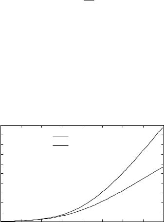
•The next term in the high SNR expansion (constant term) shows the performance degradation, in rate, of using the decorrelator bank as compared to the capacity of the channel. Figure 8.10 highlights this difference in the special case of nt = nr = n.
The above analysis is for the high SNR regime. At any fixed SNR, it is also straightforward to show that, just like the capacity, the total rate achievable by the bank of decorrelators scales linearly with the number of antennas (see Exercise 8.21).
Figure 8.10 Plot of rate achievable with the decorrelator bank for the nt = nr = 8 i.i.d. Rayleigh
fading channel. The capacity of the channel is also plotted for comparison.
70
60
Capacity
50
Decorrelator
Hz
40
/s/
bits
30
20
10
0
–10
–5
0
5
10
15
20
25
30
SNR (dB)
355
8.3 Receiver architectures
8.3.2 Successive cancellation
Figure 8.11 Decorrelator–SIC: A bank of decorrelators with successive cancellation of streams.
We have just considered a bank of separate filters to estimate the data streams. However, the result of one of the filters could be used to aid the operation of the others. Indeed, we can use the successive cancellation strategy described in the uplink capacity analysis (in Section 6.1): once a data stream is successfully recovered, we can subtract it off from the received vector and reduce the burden on the receivers of the remaining data streams. With this motivation, consider the following modification to the bank of separate receiver structures in Figure 8.8. We use the first decorrelator to decode the data stream x1m and then subtract off this decoded stream from the received vector. If the first stream is successfully decoded, then the second decorrelator has to deal only with streams x3 xnt as interference, since x1 has been correctly subtracted off. Thus, the second decorrelator projects onto the subspace orthogonal to that spanned by h3 hnt . This process is continued until the final decorrelator does not have to deal with any interference from the other data streams (assuming successful subtraction in each preceding stage). This decorrelator– SIC (decorrelator with successive interference cancellation) architecture is illustrated in Figure 8.11.
One problem with this receiver structure is error propagation: an error in decoding the kth data stream means that the subtracted signal is incorrect and this error propagates to all the streams further down, k + 1 nt. A careful analysis of the performance of this scheme is complicated, but can be made easier if we take the data streams to be well coded and the block length to be very large, so that streams are successfully cancelled with very high probability. With this assumption the kth data stream sees only down-stream interference, i.e., from the streams k + 1 nt. Thus,
Decode
Stream 1
Decorrelator 1
stream 1
Stream 2
Subtract
Decode
stream1
Decorrelator 2
stream 2
Subtract
Decode
Stream 3
y[m]
stream1, 2
Decorrelator 3
stream 3
Subtract
Decorrelator nt
Decode
Stream nt
stream
stream nt
1, 2, ..., nt –1
356
MIMO II: capacity and multiplexing architectures
˜
the corresponding projection operation (denoted by Qk) is onto a higher dimensional subspace (one orthogonal to that spanned by hk+1 hnt , as opposed to being orthogonal to the span of h1 hk−1 hk+1 hnt ). As in the calculation of the previous section, the SNR of the kth data stream is (cf. (8.44))
Pk Q˜ khk 2
(8.55)
N0
While we clearly expect this to be an improvement over the simple bank of decorrelators, let us again turn to the i.i.d. Rayleigh fading model to see this concretely. Analogous to the high SNR expansion of (8.52) in (8.53) for the simple decorrelator bank, with SIC and equal power allocation to each stream, we have
SNR
nt
Rdec−sic ≈ nmin log
nt
+ k
1 log Q˜ khk 2
(8.56)
=
Similar to our analysis of the basic decorrelator bank, we can argue that
˜ 2 '2
Qkhk 2 nr −nt +k with probability 1 (cf. Exercise 8.13), thus arriving at
!log Q˜ khk 2 " = log '22 nr −nt +k
(8.57)
Comparing this rate at high SNR with both the simple decorrelator bank and the capacity of the channel (cf. (8.53) and (8.18)), we observe the following
•The first-order term in the high SNR expansion is the same as that in the rate of the decorrelator bank and in the capacity: successive cancellation does not provide additional degrees of freedom.
•Moving to the next (constant) term, we see the performance boost in using the decorrelator–SIC over the simple decorrelator bank: the improved constant term is now equal to that in the capacity expansion. This boost in performance can be viewed as a power gain: by decoding and subtracting instead of linear nulling, the effective SNR at each stage is improved.
8.3.3Linear MMSE receiver
Limitation of the decorrelator
We have seen the performance of the basic decorrelator bank and the decorrelator–SIC. At high SNR, for i.i.d. Rayleigh fading, the basic decorrelator bank achieves the full degrees of freedom in the channel. With SIC even the constant term in the high SNR capacity expansion is achieved. What about low SNR? The performance of the decorrelator bank (both with and without the modification of successive cancellation) as compared to the capacity of the MIMO channel is plotted in Figure 8.12.
357
Figure 8.12 Performance of the decorrelator bank, with and without successive cancellation at low SNR. Here nt = nr = 8.
8.3 Receiver architectures
0.8
0.7 Without successive cancellation
With successive cancellation
0.6
0.5
Rdecorr
C88 0.4
0.3
0.2
0.1
20
30
–30
–20
–10
0
10
SNR (dB)
The main observation is that while the decorrelator bank performs well at high SNR, it is really far away from the capacity at low SNR. What is going on here?
To get more insight, let us plot the performance of a bank of matched filters, the kth filter being matched to the spatial signature hk of transmit antenna k. From Figure 8.13 we see that the performance of the bank of matched filters is far superior to the decorrelator bank at low SNR (although far inferior at high SNR).
Derivation of the MMSE receiver
The decorrelator was motivated by the fact that it completely nulls out interstream interference; in fact it maximizes the output SNR among all linear
Figure 8.13 Performance (ratio of the rate to the capacity) of the matched filter bank as compared to that of the decorrelator bank. At low SNR, the matched filter is superior. The opposite is true for the decorrelator. The channel is i.i.d. Rayleigh with nt = nr = 8.