Fundamentals Of Wireless Communication

338 MIMO II: capacity and multiplexing architectures

Comparing this expression to the waterfilling capacity in (7.10), we see the contrast between the situation when the transmitter knows the channel and when it does not. When the transmitter knows the channel, it can allocate different amounts of power in the different eigenmodes depending on their strengths. When the transmitter does not know the channel but the channel is sufficiently random, the optimal covariance matrix is identity, resulting in equal amounts of power across the eigenmodes.

8.2.2 Performance gains

The capacity, (8.16), of the MIMO fading channel is a function of the distribution of the singular values, i, of the random channel matrix H. By Jensen’s inequality, we know that

with equality if and only if the singular values are all equal. Hence, one would expect a high capacity if the channel matrix H is sufficiently random and statistically well conditioned, with the overall channel gain well distributed across the singular values. In particular, one would expect such a channel to attain the full degrees of freedom at high SNR.

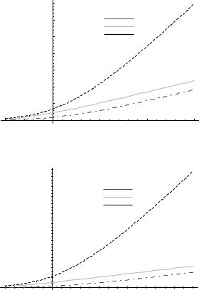
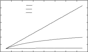
We plot the capacity for the i.i.d. Rayleigh fading model in Figure 8.2 for different numbers of antennas. Indeed, we see that for such a random channel the capacity of a MIMO system can be very large. At moderate to high SNR, the capacity of an n by n channel is about n times the capacity of a 1 by 1 system. The asymptotic slope of capacity versus SNR in dB

scale is proportional to n, which means that the capacity scales with SNR like n log SNR.

High SNR regime

The performance gain can be seen most clearly in the high SNR regime. At high SNR, the capacity for the i.i.d. Rayleigh channel is given by

for all i. Hence, the full nmin degrees of freedom is attained. In fact, further analysis reveals that

shift of the capacity versus SNR curves. At high SNR, a power gain is much less impressive than a degree-of-freedom gain.

Low SNR regime

Here we use the approximation log2 1 + x ≈ x log2 e for x small in (8.15) to get

= nrSNR log2 e bits/s/Hz

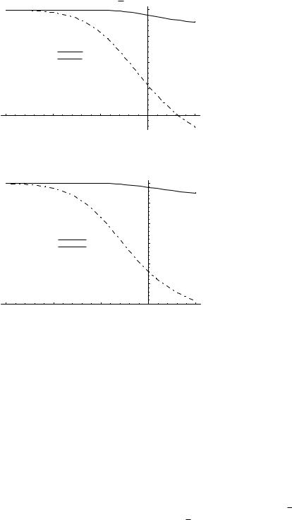
Thus, at low SNR, an nt by nr system yields a power gain of nr over a single antenna system. This is due to the fact that the multiple receive antennas can coherently combine their received signals to get a power boost. Note that increasing the number of transmit antennas does not increase the power gain since, unlike the case when the channel is known at the transmitter, transmit beamforming cannot be done to constructively add signals from the different antennas. Thus, at low SNR and without channel knowledge at the transmitter, multiple transmit antennas are not very useful: the performance of an nt by nr channel is comparable with that of a 1 by nr channel. This is illustrated in Figure 8.3, which compares the capacity of an n by n channel with that of a 1 by n channel, as a fraction of the capacity of a 1 by 1 channel. We see that at an SNR of about −20 dB, the capacities of a 1 by 4 channel and a 4 by 4 channel are very similar.

Recall from Chapter 4 that the operating SINR of cellular systems with universal frequency reuse is typically very low. For example, an IS-95 CDMA system may have an SINR per chip of −15 to −17 dB. The above observation then suggests that just simply overlaying point-to-point MIMO technology on such systems to boost up per link capacity will not provide much additional benefit than just adding antennas at one end. On the other hand, the story is different if the multiple antennas are used to perform multiple access and interference management. This issue will be revisited in Chapter 10.

Another difference between the high and the low SNR regimes is that while channel randomness is crucial in yielding a large capacity gain in the high SNR regime, it plays little role in the low SNR regime. The low SNR result above does not depend on whether the channel gains, hij , are independent or correlated.

•MISO channel with a large transmit antenna array Specializing (8.15) to the n by 1 MISO channel yields the capacity

For n = 1, the 1 by 1 fading channel (with only receiver CSI) has lower capacity than the AWGN channel; this is due to the “Jensen’s loss” (Section 5.4.5). But recall from Figure 5.20 that this loss is not large for the entire range of SNR. Increasing the number of transmit antennas has the effect of reducing the fluctuation of the instantaneous SNR

and hence reducing the Jensen’s loss, but the loss was not big to start with, hence the gain is minimal. Since the total transmit power is fixed, the multiple transmit antennas provide neither a power gain nor a gain in spatial degrees of freedom. (In a slow fading channel, the multiple transmit antennas provide a diversity gain, but this is not relevant in the fast fading scenario considered here.)

•SIMO channel with a large receive antenna array A 1 by n SIMO channel has capacity

i.e., the receive antennas provide a power gain (which increases linearly with the number of receive antennas) and the capacity increases logarithmically with the number of receive antennas. This is quite in contrast to the MISO case: the difference is due to the fact that now there is a linear increase in total received power due to a larger receive antenna array. However, the increase in capacity is only logarithmic in n; the increase in total received power is all accumulated in the single degree of freedom of the channel. There is power gain but no gain in the spatial degrees of freedom.

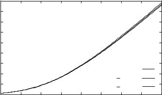
The capacities, as a function of n, are plotted for the SIMO, MISO and MIMO channels in Figure 8.6.

346 MIMO II: capacity and multiplexing architectures

limited by the antenna array aperture rather than the number of antenna elements.

8.2.3 Full CSI

We have considered the scenario when only the receiver can track the channel. This is the most interesting case in practice. In a TDD system or in an FDD system where the fading is very slow, it may be possible to track the channel matrix at the transmitter. We shall now discuss how channel capacity can be achieved in this scenario. Although channel knowledge at the transmitter does not help in extracting an additional degree-of-freedom gain, extra power gain is possible.

Capacity

The derivation of the channel capacity in the full CSI scenario is only a slight twist on the time-invariant case discussed in Section 7.1.1. At each time m, we decompose the channel matrix as Hm = Um mVm , so that the MIMO channel can be represented as a parallel channel

y˜im = im x˜im + w˜ im i = 1 nmin (8.36)

where 1m ≥ 2m ≥ ≥ nmin m are the ordered singular values of

Hm and

x˜m = V mxm

y˜m = U mym w˜ m = U mwm

We have encountered the fast fading parallel channel in our study of the single antenna fast fading channel (cf. Section 5.4.6). We allocate powers to the sub-channels based on their strength according to the waterfilling policy

with chosen so that the total transmit power constraint is satisfied:

− N0 + = P (8.38)

2i

Note that this is waterfilling over time and space (the eigenmodes). The capacity is given by

Transceiver architecture

The transceiver architecture that achieves the capacity follows naturally from the SVD-based architecture depicted in Figure 7.2. Information bits are split into nmin parallel streams, each coded separately, and then augmented by nt − nmin streams of zeros. The symbols across the streams at time m form the vector x˜ m . This vector is pre-multiplied by the matrix V m before being sent through the channel, where H m = U m m V m is the singular value decomposition of the channel matrix at time m. The output is post-multiplied by the matrix U m to extract the independent streams, which are then separately decoded. The power allocated to each stream is time-dependent and is given by the waterfilling formula (8.37), and the rates are dynamically allocated accordingly. If an AWGN capacity-achieving code is used for each stream, then the entire system will be capacity-achieving for the MIMO channel.

Performance analysis

Let us focus on the i.i.d. Rayleigh fading model. Since with probability 1, the random matrix HH has full rank (Exercise 8.12), and is, in fact, wellconditioned (Exercise 8.14), it can be shown that at high SNR, the waterfilling strategy allocates an equal amount of power P/nmin to all the spatial modes, as well as an equal amount of power over time. Thus,

where SNR = P/N0. If we compare this to the capacity (8.16) with only receiver CSI, we see that the number of degrees of freedom is the same nmin but there is a power gain of a factor of nt/nmin when the transmitter can track the channel. Thus, whenever there are more transmit antennas then receive antennas, there is a power boost of nt/nr from having transmitter CSI. The reason is simple. Without channel knowledge at the transmitter, the transmit energy is spread out equally across all directions in nt . With transmitter CSI, the energy can now be focused on only the nr non-zero eigenmodes, which form a subspace of dimension nr inside nt . For example, with nr = 1, the capacity with only receiver CSI is

while the high SNR capacity when there is full CSI is