Fundamentals Of Wireless Communication

AWGN channel. Thus, we can use the encoding and decoding procedures for the code designed for the uplink AWGN channel. In particular, to achieve the maximum sum rate, we can use orthogonal multiple access: this means that the codes designed for the point-to-point AWGN channel can be used. Contrast this with the case when only the receiver has CSI, where we have shown that orthogonal multiple access is strictly suboptimal for fading channels. Note that this argument on the optimality of orthogonal multiple access holds regardless of whether the users have symmetric fading statistics.

In the case of the symmetric uplink considered here, the optimal power allocation takes on a particularly simple structure. To derive it, let us consider the optimization problem (6.42), but with the individual power constraints in (6.43) relaxed and replaced by a total power constraint:

and for a given total power Kk=1 Pk allocated to the th sub-channel, this quantity is maximized by giving all that power to the user with the strongest channel gain. Thus, the solution of the optimization problem (6.42) subject to the constraint (6.44) is that at each time, allow only the user with the best channel to transmit. Since there is just one user transmitting at any time, we have reduced to a point-to-point problem and can directly infer from our discussion in Section 5.4.6 that the best user allocates its power according to the waterfilling policy. More precisely, the optimal power allocation policy is

where is chosen to meet the sum power constraint (6.44). Taking the number of coherence periods L → and appealing to the ergodicity of the fading process, we get the optimal capacity-achieving power allocation strategy, which allocates powers to the users as a function of the joint channel state h = h1 hK :

249 6.3 Uplink fading channel

with chosen to satisfy the power constraint

k=1

(Rigorously speaking, this formula is valid only when there is exactly one user with the strongest channel. See Exercise 6.16 for the generalization to the case when multiple users can have the same fading state.) The resulting sum capacity is

where k h is the index of the user with the strongest channel at joint channel state h.

We have derived this result assuming a total power constraint on all the users, but by symmetry, the power consumption of all the users is the same under the optimal solution (recall that we are assuming independent and identical fading processes across the users here). Therefore the individual power constraints in (6.43) are automatically satisfied and we have solved the original problem as well.

This result is the multiuser generalization of the idea of opportunistic communication developed in Chapter 5: resource is allocated at the times and to the user whose channel is good.

When one attempts to generalize the optimal power allocation solution from the point-to-point setting to the multiuser setting, it may be tempting to think of “users” as a new dimension, in addition to the time dimension, over which dynamic power allocation can be performed. This may lead us to guess that the optimal solution is waterfilling over the joint time/user space. This, as we have already seen, is not the correct solution. The flaw in this reasoning is that having multiple users does not provide additional degrees of freedom in the system: the users are just sharing the time/frequency degrees of freedom already existing in the channel. Thus, the optimal power allocation problem should really be thought of as how to partition the total resource (power) across the time/frequency degrees of freedom and how to share the resource across the users in each of those degrees of freedom. The above solution says that from the point of view of maximizing the sum capacity, the optimal sharing is just to allocate all the power to the user with the strongest channel on that degree of freedom.

We have focused on the sum capacity in the symmetric case where users have identical channel statistics and power constraints. It turns out that in the asymmetric case, the optimal strategy to achieve sum capacity is still to have one user transmitting at a time, but the criterion of choosing which user is different. This problem is analyzed in Exercise 6.15. However, in the asymmetric case, maximizing the sum rate may not be the appropriate objective,

turn to the analogous situation in the downlink where the single transmitter tracks all the channels of the users it is communicating to (the users continue to track their individual channels). As in the uplink, we can allocate powers to the users as a function of the channel fade level. To see the effect, let us continue focusing on sum capacity. We have seen that without fading, the sum capacity is achieved by transmitting only to the best user. Now as the channels vary, we can pick the best user at each time and further allocate it an appropriate power, subject to a constraint on the average power. Under this strategy, the downlink channel reduces to a point-to-point channel with the channel gain distributed as

max hk 2

k=1 K

The optimal power allocation is the, by now familiar, waterfilling solution:

where h = h1 hK t is the joint fading state and > 0 is chosen such that the average power constraint is met. The optimal strategy is exactly the same as in the sum capacity of the uplink. The sum capacity of the downlink is:

6.5 Frequency-selective fading channels

The extension of the flat fading analysis in the uplink and the downlink to underspread frequency-selective fading channels is conceptually straightforward. As we saw in Section 5.4.7 in the point-to-point setting, we can think of the underspread channel as a set of parallel sub-carriers over each coherence time interval and varying independently from one coherence time interval to the other. We can see this constructively by imposing a cyclic prefix to all the transmit signals; the cyclic prefix should be of length that is larger than the largest multipath delay spread that we are likely to encounter among the different users. Since this overhead is fixed, the loss is amortized when communicating over a long block length.

We can apply exactly the same OFDM transformation to the multiuser channels. Thus on the nth sub-carrier, we can write the uplink channel as

k=1

253 6.6 Multiuser diversity

where d k i , h k i and y i , respectively, represent the DFTs of the transsequence of user k, of the channel and of the received sequence at

The flat fading uplink channel can be viewed as a set of parallel multiuser sub-channels, one for each coherence time interval. With full CSI, the optimal strategy to maximize the sum rate in the symmetric case is to allow only the user with the best channel to transmit at each coherence time interval. The frequency-selective fading uplink channel can also be viewed as a set of parallel multiuser sub-channels, one for each sub-carrier and each coherence time interval. Thus, the optimal strategy is to allow the best user to transmit on each of these sub-channels. The power allocated to the best user is waterfilling over time and frequency. As opposed to the flat fading case, multiple users can now transmit at the same time, but over different sub-carriers. Exactly the same comments apply to the downlink.

6.6 Multiuser diversity

6.6.1 Multiuser diversity gain

Let us consider the sum capacity of the uplink and downlink flat fading channels (see (6.49) and (6.54), respectively). Each can be interpreted as the waterfilling capacity of a point-to-point link with a power constraint equal to the total transmit power (in the uplink this is equal to KP and in the downlink it is equal to P), and a fading process whose magnitude varies as maxk hk m . Compared to a system with a single transmitting user, the multiuser gain comes from two effects:

1.the increase in total transmit power in the case of the uplink;

2.the effective channel gain at time m that is improved from h1 m 2 to max1≤k≤K hk m 2.

The first effect already appeared in the uplink AWGN channel and also in the fading channel with channel side information only at the receiver. The second effect is entirely due to the ability to dynamically schedule resources among the users as a function of the channel state.

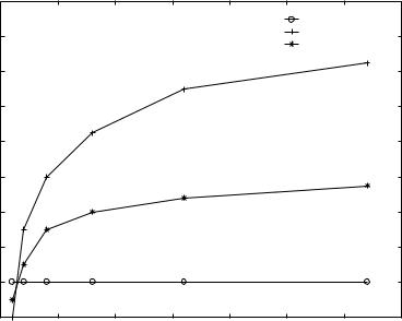
The sum capacity of the uplink Rayleigh fading channel with full CSI is plotted in Figure 6.11 for different numbers of users. The performance curves are plotted as a function of the total SNR = KP/N0 so as to focus on the second effect. The sum capacity of the channel with only CSI at the receiver is also plotted for different numbers of users. The capacity of the point-to-point AWGN channel with received power KP (which is also the sum capacity of a K-user uplink AWGN channel) is shown as a baseline. Figure 6.12 focuses on the low SNR regime.

256 Multiuser capacity and opportunistic communication

Section 2.4 that, Rician fading models the situation when there is a strong specular line-of-sight path plus many small reflected paths. The parameter is defined as the ratio of the energy in the specular line-of-sight path to the energy in the diffused components. Because of the line-of-sight component, the Rician fading distribution is less “random” and has a lighter tail than the Rayleigh distribution with the same average channel gain. As a consequence, it can be seen that the multiuser diversity gain is significantly smaller in the Rician case compared to the Rayleigh case (Exercise 6.21).

6.6.2 Multiuser versus classical diversity

We have called the above explained phenomenon multiuser diversity. Like the diversity techniques discussed in Chapter 3, multiuser diversity also arises from the existence of independently faded signal paths, in this case from the multiple users in the network. However, there are several important differences. First, the main objective of the diversity techniques in Chapter 3 is to improve the reliability of communication in slow fading channels; in contrast, the role of multiuser diversity is to increase the total throughput over fast fading channels. Under the sum-capacity-achieving strategy, a user has no guarantee of a high rate in any particular slow fading state; only by averaging over the variations of the channel is a high long-term average throughput attained. Second, while the diversity techniques are designed to counteract the adverse effect of fading, multiuser diversity improves system performance by exploiting channel fading: channel fluctuations due to fading ensure that with high probability there is a user with a channel strength much larger than the mean level; by allocating all the system resources to that user, the benefit of this strong channel is fully capitalized. Third, while the diversity techniques in Chapter 3 pertain to a point-to-point link, the benefit of multiuser diversity is system-wide, across the users in the network. This aspect of multiuser diversity has ramifications on the implementation of multiuser diversity in a cellular system. We will discuss this next.

6.7 Multiuser diversity: system aspects

The cellular system requirements to extract the multiuser diversity benefits are:

•the base-station has access to channel quality measurements: in the downlink, we need each receiver to track its own channel SNR, through say a common downlink pilot, and feed back the instantaneous channel quality to the base-station (assuming an FDD system); and in the uplink, we need transmissions from the users so that their channel qualities can be tracked;

•the ability of the base-station to schedule transmissions among the users as well as to adapt the data rate as a function of the instantaneous channel quality.

These features are already present in the designs of many third-generation systems. Nevertheless, in practice there are several considerations to take into account before realizing such gains. In this section, we study three main hurdles towards a system implementation of the multiuser diversity idea and some prominent ways of addressing these issues.

1.Fairness and delay To implement the idea of multiuser diversity in a real system, one is immediately confronted with two issues: fairness and delay. In the ideal situation when users’ fading statistics are the same, the strategy of communicating with the user having the best channel maximizes not only the total throughput of the system but also that of individual users. In reality, the statistics are not symmetric; there are users who are closer to the base-station with a better average SNR; there are users who are stationary and some that are moving; there are users who are in a rich scattering environment and some with no scatterers around them. Moreover, the strategy is only concerned with maximizing long-term average throughputs; in practice there are latency requirements, in which case the average throughput over the delay time-scale is the performance metric of interest. The challenge is to address these issues while at the same time exploiting the multiuser diversity gain inherent in a system with users having independent, fluctuating channel conditions. As a case study, we will look at one particular scheduler that harnesses multiuser diversity while addressing the real-world fairness and delay issues.

2.Channel measurement and feedback One of the key system requirements to harness multiuser diversity is to have scheduling decisions by the basestation be made as a function of the channel states of the users. In the uplink, the base-station has access to the user transmissions (over trickle channels which are used to convey control information) and has an estimate of the user channels. In the downlink, the users have access to their channel states but need to feedback these values to the base-station. Both the error in channel state measurement and the delay in feeding it back constitute a significant bottleneck in extracting the multiuser diversity gains.

3.Slow and limited fluctuations We have observed that the multiuser diversity gains depend on the distribution of channel fluctuations. In particular, larger and faster variations in a channel are preferred over slow ones. However, there may be a line-of-sight path and little scattering in the environment, and hence the dynamic range of channel fluctuations may be small. Further, the channel may fade very slowly compared to the delay constraints of the application so that transmissions cannot wait until the channel reaches its peak. Effectively, the dynamic range of channel fluctuations is small within the time-scale of interest. Both are important