Fundamentals Of Wireless Communication

459 10.3 Downlink with multiple transmit antennas

Putting the two constraints (10.51) and (10.52) together, we get

which implies that the maximum rate of reliable communication is, at most,

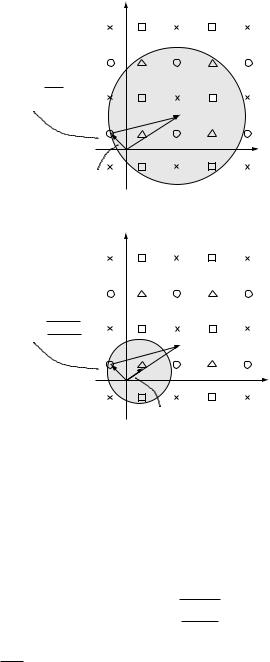
This yields an upper bound on the rate of reliable communication. Moreover, it can be shown that if the MK constellation points are independently and uniformly distributed on the domain, then with high probability, communication is reliable if condition (10.51) holds and the average power constraint is satisfied if condition (10.52) holds. Thus, the rate (10.54) is also achievable. The proof of this is along the lines of the argument in Appendix B.5.2, where the achievability of the AWGN capacity is shown.

Observe that the rate (10.54) is close to the AWGN capacity 1/2 log 1 + P/2 at high SNR. However, the scheme is strictly suboptimal at finite SNR. In fact, it achieves zero rate if the SNR is below 0 dB. How can the performance of this scheme be improved?

Performance enhancement via MMSE estimation

The performance of the above scheme is limited by the two constraints (10.51) and (10.52). To meet the average power constraint, the density of replication cannot be reduced beyond (10.52). On the other hand, constraint (10.51) is a direct consequence of the nearest neighbor decoding rule, and this rule is in fact suboptimal for the problem at hand. To see why, consider the case when the

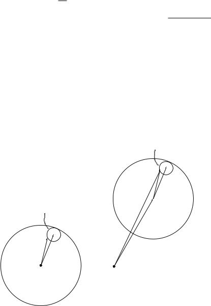
interference vector s is 0 and the noise variance 2 is significantly larger than

√

P. In this case, the transmitted vector x1 is roughly at a distance NP from the origin while the received vector y is at a distance N P + 2 , much further

(Figure 10.22). Without using this prior information, the transmitted vector is

thought of by the receiver as anywhere in a large uncertainty sphere of radius

√

N2 around y and the extended constellation points have to be spaced that far apart to avoid confusion. By making use of the prior information, the size of the uncertainty sphere can be reduced. In particular, we can consider a linear estimate y of x1. By the law of large numbers, the squared error in the estimate is

The discussion of such codes is beyond the scope of this book. The design problem, however, simplifies in the low SNR regime. We discuss this below.

Low SNR: opportunistic orthogonal coding

In the infinite bandwidth channel, the SNR per degree of freedom is zero and we can use this as a concrete channel to study the nature of precoding at low SNR. Consider the infinite bandwidth real AWGN channel with additive interference s t modelled as real white Gaussian (with power spectral density Ns/2) and known non-causally to the transmitter. The interference is independent of both the background real white Gaussian noise and the real transmit signal, which is power constrained, but not bandwidth constrained. Since the interference is known non-causally only to the transmitter, the minimumb/N0 for reliable communication on this channel can be no smaller than that in the plain AWGN channel without interference; thus a lower bound on the minimum b/N0 is −1 59 dB.

We have already seen for the AWGN channel (cf. Section 5.2.2 and Exercises 5.8 and 5.9) that orthogonal codes achieve the capacity in the infinite bandwidth regime. Equivalently, orthogonal codes achieve the minimum b/N0 of −1 59 dB over the AWGN channel. Hence, we start with an orthogonal set of codewords representing M messages. Each of the codewords is replicated K times so that the overall constellation with MK vectors forms an orthogonal set. Each of the M messages corresponds to a set of K orthogonal signals. To convey a specific message, the encoder transmits that signal, among the set of K orthogonal signals corresponding to the message selected, that is closest to the interference s t , i.e., the one that has the largest correlation with the s t . This signal is the constellation point to which s t is quantized. Note that, in the general scheme, the signal qu s − s is transmitted, but since → 0 in the low SNR regime, we are transmitting qu s itself.

An equivalent way of seeing this scheme is as opportunistic pulse position modulation: classical PPM involves a pulse that conveys information based on the position when it is not zero. Here, every K of the pulse positions corresponds to one message and the encoder opportunistically chooses the position of the pulse among the K possible pulse positions (once the desired message to be conveyed is picked) where the interference is the largest.

The decoder first picks the most likely position of the transmit pulse (among the MK possible choices) using the standard largest amplitude detector. Next, it picks the message corresponding to the set in which the most likely pulse occurs. Choosing K large allows the encoder to harness the opportunistic gains afforded by the knowledge of the additive interference. On the other hand, decoding gets harder as K increases since the number of possible pulse positions, MK, grows with K. An appropriate choice of K as a function of the number of messages, M, and the noise and interference powers, N0 and Ns respectively, trades off the opportunistic gains on the one hand with

465 10.3 Downlink with multiple transmit antennas

the increased difficulty in decoding on the other. This tradeoff is evaluated in Exercise 10.16 where we see that the correct choice of K allows the opportunistic orthogonal codes to achieve the infinite bandwidth capacity of the AWGN channel without interference. Equivalently, the minimum b/N0 is the same as that in the plain AWGN channel and is achieved by opportunistic orthogonal coding.

10.3.4 Precoding for the downlink

We now apply the precoding technique to the downlink channel. We first start with the single transmit antenna case and then discuss the multiple antenna case.

Single transmit antenna

Consider the two-user downlink channel with a single transmit antenna:

where wk m 0 N0 . Without loss of generality, let us assume that user 1 has the stronger channel: h1 2 ≥ h2 2. Write x m = x1 m + x2 m , where xk m is the signal intended for user k k = 1 2. Let Pk be the power allocated to user k. We use a standard i.i.d. Gaussian codebook to encode information for user 2 in x2 m . Treating x2 m as interference that is known at the transmitter, we can apply Costa precoding for user 1 to achieve a rate of

the capacity of an AWGN channel for user 1 with x2 m completely absent. What about user 2? It can be shown that x1 m can be made to appear like independent Gaussian noise to user 2. (See Exercise 10.17.) Hence, user 2 gets a reliable data rate of

Since we have assumed that user 1 has the stronger channel, these same rates can in fact be achieved by superposition coding and decoding (cf. Section 6.2): we superimpose independent i.i.d. Gaussian codebook for user 1 and 2, with user 2 decoding the signal x2 m treating x1 m as Gaussian noise, and user 1 decoding the information for user 2, canceling it off, and then decoding the information intended for it. Thus, precoding is another approach to achieve rates on the boundary of the capacity region in the single antenna downlink channel.

466 MIMO IV: multiuser communication

Superposition coding is a receiver-centric scheme: the base-station simply adds the codewords of the users while the stronger user has to do the decoding job of both the users. In contrast, precoding puts a substantial computational burden on the base-station with receivers being regular nearest neighbor decoders (though the user whose signal is being precoded needs to decode the extended constellation, which has more points than the rate would entail). In this sense we can think of precoding as a transmitter-centric scheme.

However, there is something curious about this calculation. The precoding strategy described above encodes information for user 1 treating user 2’s signal as known interference. But certainly we can reverse the role of user 1 and user 2, and encode information for user 2, treating user 1’s signal as

But these rates cannot be achieved by superposition coding/decoding under the power allocations P1 P2: the weak user cannot remove the signal intended for the strong user. Is this rate tuple then outside the capacity region? It turns out that there is no contradiction and this rate pair is strictly contained inside the capacity region (Exercise 10.19).

In this discussion, we have restricted ourselves to just two users, but the extension to K users is obvious. See Exercise 10.19.

Multiple transmit antennas

We now return to the scenario of real interest, multiple transmit antennas (10.31):

The precoding technique can be applied to upgrade the performance of the linear beamforming technique described in Section 10.3.2. Recall from (10.35), the transmitted signal is

k=1

where x˜km is the signal for user k and uk is its transmit beamforming vector. The received signal of user k is given by

j>k

467 10.3 Downlink with multiple transmit antennas

where SINRk is the effective signal-to-interference-plus-noise ratio after precoding:

Here Pj is the power allocated to user j. Observe that unlike the single transmit antenna case, this performance may not be achievable by superposition coding/decoding.

For linear beamforming strategies, an interesting uplink–downlink duality is identified in Section 10.3.2. We can use the downlink transmit signatures (denoted by u1 uK) to be the same as the receive filters in the dual uplink channel (10.40) and the same SINR for the users can be achieved in both the uplink and the downlink with appropriate user power allocations such that the sum of these power allocations is the same for both the uplink and the downlink. We now extend this observation to a duality between transmit beamforming with precoding in the downlink and receive beamforming with SIC in the uplink.

Specifically, suppose we use Costa precoding in the downlink and SIC in the uplink, and the transmit signatures of the users in the downlink are the same as the receive filters of the users in the uplink. Then it turns out that the same set SINR of the users can be achieved by appropriate user power allocations in the uplink and the downlink and, further, the sum of these power allocations is the same. This duality holds provided that the order of SIC in the uplink is the reverse of the Costa precoding order in the downlink. For example, in the Costa precoding above we employed the order 1 K; i.e., we precoded the user k signal so as to cancel the interference from the signals of users 1 k − 1. For this duality to hold, we need to reverse this order in the SIC in the uplink; i.e., the users are successively canceled in the order K 1 (with user k seeing no interference from the canceled user signals K K − 1 k + 1).

The derivation of this duality follows the same lines as for linear strategies and is done in Exercise 10.20. Note that in this SIC ordering, user 1 sees the least uncanceled interference and user K sees the most. This is exactly the opposite to that under the Costa precoding strategy. Thus, we see that in this duality the ordering of the users is reversed. Identifying this duality facilitates the computation of good transmit filters in the downlink. For example, we know that in the uplink the optimal filters for a given set of powers are MMSE filters; the same filters can be used in the downlink transmission.