Fundamentals Of Wireless Communication

528 Appendix B Information theory from first principles

is now reduced to finding the input distribution on x to maximize h y subject to a second moment constraint on x. To solve this problem, we use a key fact about Gaussian random variables: they are differential entropy maximizers. More precisely, given a constraint E u2 ≤ A on a random variable u, the distribution u is 0 A maximizes the differential entropy h u. (See Exercise B.6 for a proof of this fact.) Applying this to our problem, we see that the second moment constraint of P on x translates into a second moment constraint of P + 2 on y. Thus, h y is maximized when y is0 P + 2 , which is achieved by choosing x to be 0 P. Thus, the capacity of the Gaussian channel is

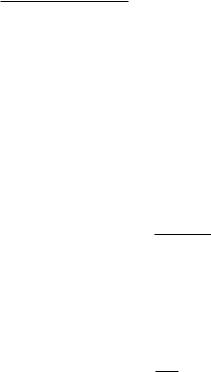
agreeing with the result obtained via the heuristic sphere-packing derivation in Section 5.1. A capacity-achieving code can be obtained by choosing each component of each codeword i.i.d. 0 P. Each codeword is therefore

isotropically distributed, and, by the law of large numbers, with high probabil-

√

ity lies near the surface of the sphere of radius NP. Since in high dimensions most of the volume of a sphere is near its surface, this is effectively the same as picking each codeword uniformly from the sphere.

where w is 0 N0 . There is an average power constraint of P per (complex) symbol. One way to derive the capacity of this channel is to think of each use of the complex channel as two uses of a real AWGN channel, with SNR = P/2/ N0/2 = P/N0. Hence, the capacity of the channel is

Alternatively we may just as well work directly with the complex channel and the associated complex random variables. This will be useful when we deal with other more complicated wireless channel models later on. To this end, one can think of the differential entropy of a complex random variable x as that of a real random vector x x. Hence, if w is 0 N0 , h w = h w + h w = log eN0 . The mutual information I x y of the complex AWGN channel y = x + w is then

With a power constraint E x 2 ≤ P on the complex input x, y is constrained to satisfy E y 2 ≤ P + N0. Here, we use an important fact: among all complex random variables, the circular symmetric Gaussian random variable maximizes the differential entropy for a given second moment constraint. (See Exercise B.7.) Hence, the capacity of the complex Gaussian channel is

which is the same as Eq. (5.11).

B.5 Sphere-packing interpretation

In this section we consider a more precise version of the heuristic spherepacking argument in Section 5.1 for the capacity of the real AWGN channel. Furthermore, we outline how the capacity as predicted by the sphere-packing argument can be achieved. The material here is particularly useful when we discuss precoding in Chapter 10.

B.5.1 Upper bound

Consider transmissions over a block of N symbols, where N is large. Suppose we use a code consisting of equally likely codewords x1 x . By the law of large numbers, the N -dimensional received vector y = x + w

will with high probability lie approximately5 within a y-sphere of radius

N P + 2 , so without loss of generality we need only to focus on what happens inside this y-sphere. Let i be the part of the maximum-likelihood decision region for xi within the y-sphere. The sum of the volumes of the i is equal to Vy, the volume of the y-sphere. Given this total volume, it can be shown, using the spherical symmetry of the Gaussian noise distribution, that the error probability is lower bounded by the (hypothetical) case when thei are all perfect spheres of equal volume Vy/ . But by the law of large

numbers, the received vector y lies near the surface of a noise sphere of radius

√

N 2 around the transmitted codeword. Thus, for reliable communication, Vy/ should be no smaller than the volume Vw of this noise sphere, otherwise even in the ideal case when the decision regions are all spheres of equal volume, the error probability will still be very large. Hence, the number of

5To make this and other statements in this section completely rigorous, appropriate and ( have to be added.

1/pN ). In terms of the data rate R bits per symbol time, this means that as long as

then reliable communication is possible.

Both the upper bound and the achievability arguments are based on calculating the ratio of volumes of spheres. The ratio is the same in both cases, but the spheres involved are different. The sphere-packing picture in Figure B.5 corresponds to the following decomposition of the capacity expression:

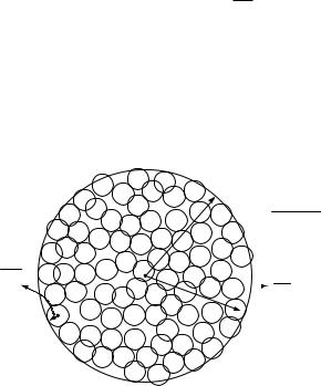
with the volume of the y-sphere proportional to 2Nh y and the volume of the noise sphere proportional to 2Nh y x . The picture in Figure B.6, on the other hand, corresponds to the decomposition:

with the volume of the x-sphere proportional to 2Nh x . Conditional on y, x is

N y mmse2 , where = P/ P + 2 is the coefficient of the MMSE estimator of x given y, and

2 = P 2

mmse P + 2

is the MMSE estimation error. The radius of the uncertainty sphere considered

above is N mmse2 and its volume is proportional to 2Nh x y . In fact the proposed receiver, which finds the nearest codeword to y, is motivated

precisely by this decomposition. In this picture, then, the AWGN capacity formula is being interpreted in terms of the number of MMSE error spheres that can be packed inside the x-sphere.

B.6 Time-invariant parallel channel

Consider the parallel channel (cf. (5.33):

subject to an average power per sub-carrier constraint of P (cf. (5.37)):

E ˜ i 2 ≤ NcP (B.54) d

533 B.7 Capacity of the fast fading channel

0 Nc − 1. Thus, computing the capacity in (B.55) is reduced to a power

The solution to this optimization problem is waterfilling and is described in

Section 5.3.3.

B.7 Capacity of the fast fading channel

B.7.1 Scalar fast fading channnel

Ideal interleaving

The fast fading channel with ideal interleaving is modeled as follows:

where the channel coefficients h m are i.i.d. in time and independent of the i.i.d. 0 N0 additive noise w m. We are interested in the situation when the receiver tracks the fading channel, but the transmitter only has access to the statistical characterization; the receiver CSI scenario. The capacity of the

power-constrained fast fading channel with receiver CSI can be written as, by viewing the receiver CSI as part of the output of the channel,

px x2 ≤P

Since the fading channel h is independent of the input, I x h = 0. Thus, by the chain rule of mutual information (see (B.18)),

Conditioned on the fading coefficient h, the channel is simply an AWGN one, with SNR equal to P h 2/N0, where we have denoted the transmit power constraint by P. The optimal input distribution for a power constrained AWGN channel is , regardless of the operating SNR. Thus, the maximizing input distribution in (B.62) is 0 P. With this input distribution,

where the average is over the stationary distribution of the fading channel.

Stationary ergodic fading

The above derivation hinges on the i.i.d. assumption on the fading process h m. Yet in fact (B.64) holds as long as h m is stationary and ergodic. The alternative derivation below is more insightful and valid for this more general setting.

We first fix a realization of the fading process h m. Recall from (B.20) that the rate of reliable communication is given by the average rate of flow of mutual information:

for almost all realizations of the fading process h m. This yields the same expression of capacity as in (B.64).

B.7.2 Fast fading MIMO channel

We have only considered the scalar fast fading channel so far; the extension of the ideas to the MIMO case is very natural. The fast fading MIMO channel with ideal interleaving is (cf. (8.7))

where the channel H is i.i.d. in time and independent of the i.i.d. additive noise, which is 0 N0Inr . There is an average total power constraint of P on the transmit signal. The capacity of the fast fading channel with receiver CSI is, as in (B.62),

px x 2 ≤P

The observation in (B.63) holds here as well, so the capacity calculation is based on the conditional mutual information Ix y H . If we fix the MIMO channel at a specific realization, we have

To proceed, we use the following fact about Gaussian random vectors: they are entropy maximizers. Specifically, among all n-dimensional complex random vectors with a given covariance matrix K, the one that maximizes the differential entropy is complex circular-symmetric jointly Gaussian 0 K (Exercise B.8). This is the vector extension of the result that Gaussian random variables are entropy maximizers for a fixed variance constraint. The corresponding maximum value is given by

If the covariance of x is Kx and the channel is H = H, then the covariance of y is

Calculating the corresponding maximal entropy of y (cf. (B.71)) and substituting in (B.70), we see that

536 Appendix B Information theory from first principles

with equality if x is 0 Kx . This means that even if the transmitter does not know the channel, there is no loss of optimality in choosing the input to be .

Finally, the capacity of the fast fading MIMO channel is found by averaging (B.73) with respect to the stationary distribution of H and choosing the appropriate covariance matrix subject to the power constraint:

Just as in the scalar case, this result can be generalized to any stationary and ergodic fading process Hm.

B.8 Outage formulation

entries), is random but not varying with time. The additive noise is i.i.d.0 N0 and independent of H.

If there is a positive probability, however small, that the entries of H are small, then the capacity of the channel is zero. In particular, the capacity of the i.i.d. Rayleigh slow fading MIMO channel is zero. So we focus on characterizing the -outage capacity: the largest rate of reliable communication such that the error probability is no more than . We are aided in this study by viewing the slow fading channel in (B.75) as a compound channel.

The basic compound channel consists of a collection of DMCs p y x,& with the same input alphabet and the same output alphabet and parameterized by . Operationally, the communication between the transmitter and the receiver is carried out over one specific channel based on the (arbitrary) choice of the parameter from the set &. The transmitter does not know the value of but the receiver does. The capacity is the largest rate at which a single coding strategy can achieve reliable communication regardless of which is chosen. The corresponding capacity achieving strategy is said to be universal over the class of channels parameterized by &. An important result in information theory is the characterization of the capacity

Here, the mutual information I x y signifies that the conditional distribution of the output symbol y given the input symbol x is given by the

channel p y x . The characterization of the capacity in (B.76) offers a natural interpretation: there exists a coding strategy, parameterized by the input distribution px, that achieves reliable communication at a rate that is the minimum mutual information among all the allowed channels. We have considered only discrete input and output alphabets, but the generalization to continuous input and output alphabets and, further, to cost constraints on the input follows much the same line as our discussion in Section B.4.1. The tutorial article [69] provides a more comprehensive introduction to compound channels.

We can view the slow fading channel in (B.75) as a compound channel parameterized by H. In this case, we can simplify the parameterization of coding strategies by the input distribution px: for any fixed H and channel input distribution px with covariance matrix Kx, the corresponding mutual information

Equality holds when px is 0 Kx (see Exercise B.8). Thus we can reparameterize a coding strategy by its corresponding covariance matrix (the input distribution is chosen to be with zero mean and the corresponding covariance). For every fixed covariance matrix Kx that satisfies the power constraint on the input, we can reword the compound channel result in (B.76) as follows. Over the slow fading MIMO channel in (B.75), there exists a universal coding strategy at a rate R bits/s/Hz that achieves reliable communication over all channels H which satisfy the property

Furthermore, no reliable communication using the coding strategy parameterized by Kx is possible over channels that are in outage: that is, they do not satisfy the condition in (B.78). We can now choose the covariance matrix, subject to the input power constraints, such that we minimize the probability of outage. With a total power constraint of P on the transmit signal, the outage probability when communicating at rate R bits/s/Hz is

The -outage capacity is now the largest rate R such that poutmimo ≤ .

By restricting the number of receive antennas nr to be 1, this discussion also characterizes the outage probability of the MISO fading channel. Further, restricting the MIMO channel H to be diagonal we have also characterized the outage probability of the parallel fading channel.