Fundamentals Of Wireless Communication

1

0.9

0.8

0.7

0.6

H(p) 0.5

0.4

0.3

0.2

0.1

0

p

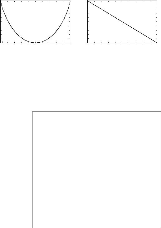
Figure B.3 The binary entropy function.

The function H · is called the binary entropy function, and is plotted in Figure B.3. It attains its maximum value of 1 at p = 1/2, and is zero when p = 0 or p = 1. Note that we never mentioned the actual values x takes on; the amount of uncertainty depends only on the probabilities.

Let us now consider two random variables x and y. The joint entropy of x and y is defined to be

The entropy of x conditional on y = j is naturally defined to be

i

This can be interpreted as the amount of uncertainty left in x after observing that y = j. The conditional entropy of x given y is the expectation of this quantity, averaged over all possible values of y:

The quantity H x y can be interpreted as the average amount of uncertainty left in x after observing y. Note that

This has a natural interpretation: the total uncertainty in x and y is the sum of the uncertainty in x plus the uncertainty in y conditional on x. This is called the chain rule for entropies. In particular, if x and y are independent, H x y = H x and hence H x y = H x + H y . One would expect that conditioning reduces uncertainty, and in fact it can be shown that

with equality if and only if x and y are independent. (See Exercise B.2.) Hence,

with equality if and only if x and y are independent.

The quantity H x −H x y is of special significance to the communication problem at hand. Since H x is the amount of uncertainty in x before observing y, this quantity can be interpreted as the reduction in uncertainty of x from the observation of y, i.e., the amount of information in y about x. Similarly, H y − H y x can be interpreted as the reduction in uncertainty of y from the observation of x. Note that

So if one defines

then this quantity is symmetric in the random variables x and y. I x y is called the mutual information between x and y. A consequence of (B.10) is that the mutual information I x y is a non-negative quantity, and equal to zero if and only if x and y are independent.

We have defined the mutual information between scalar random variables, but the definition extends naturally to random vectors. For example, I x1 x2 y should be interpreted as the mutual information between the ran-

dom vector x1 x2 and y, i.e., I x1 x2 y = H x1 x2 −H x1 x2 y . One can also define a notion of conditional mutual information:

521 B.3 Noisy channel coding theorem

I x1 x2 y = H x1 x2 − H x1 x2 y

=H x1 + H x2 x1 − H x1 y + H x2 x1 y

=I x1 y + I x2 y x1

This is the chain rule for mutual information:

In words: the information that x1 and x2 jointly provide about y is equal to the sum of the information x1 provides about y plus the additional information x2 provides about y after observing x1. This fact is very useful in Chapters 7 to 10.

B.3 Noisy channel coding theorem

Let us now go back to the communication problem shown in Figure B.2. We convey one of equally likely messages by mapping it to its N -length codeword in the code = x1 x . The input to the channel is then an N -dimensional random vector x, uniformly distributed on the codewords of . The output of the channel is another N -dimensional vector y.

B.3.1 Reliable communication and conditional entropy

To decode the transmitted message correctly with high probability, it is clear that the conditional entropy H x y has to be close to zero3. Otherwise, there is too much uncertainty in the input, given the output, to figure out what the right message is. Now,

3This statement can be made precise in the regime of large block lengths using Faro’s inequality.

i.e., the uncertainty in x subtracting the reduction in uncertainty in x by observing y. The entropy Hx is equal to log = NR, where R is the data rate. For reliable communication, Hx y ≈ 0, which implies

Intuitively: for reliable communication, the rate of flow of mutual information across the channel should match the rate at which information is generated. Now, the mutual information depends on the distribution of the random input x, and this distribution is in turn a function of the code . By optimizing over all codes, we get an upper bound on the reliable rate of communication:

B.3.2 A simple upper bound

The optimization problem (B.21) is a high-dimensional combinatorial one and is difficult to solve. Observe that since the input vector x is uniformly distributed on the codewords of , the optimization in (B.21) is over only a subset of possible input distributions. We can derive a further upper bound by relaxing the feasible set and allowing the optimization to be over all input distributions:

m=1

The inequality in (B.24) follows from (B.11) and the equality in (B.25) comes from the memoryless property of the channel. Equality in (B.24) is attained if the output symbols are independent over time, and one way to achieve this is to make the inputs independent over time. Hence,

523 B.3 Noisy channel coding theorem

Thus, the optimizing problem over input distributions on the N -length block reduces to an optimization problem over input distributions on single symbols.

B.3.3 Achieving the upper bound

To achieve this upper bound ¯ , one has to find a code whose mutual infor-

C

mation x y per symbol is close to ¯ such that (B.20) is satisfied.

I /N C and

A priori it is unclear if such a code exists at all. The cornerstone result of information theory, due to Shannon, is that indeed such codes exist if the block length N is chosen sufficiently large.

Theorem B.1 (Noisy channel coding theorem [109]) Consider a discrete memoryless channel with input symbol x and output symbol y. The capacity of the channel is

px

Shannon’s proof of the existence of optimal codes is through a randomization argument. Given any symbol input distribution px, we can randomly generate a code with rate R by choosing each symbol in each codeword independently according to px. The main result is that with the rate as in (B.20), the code with large block length N satisfies, with high probability,

In particular, by choosing codewords according to the distribution px that maximizes I x y , the maximum reliable rate is achieved. The smaller the desired error probability, the larger the block length N has to be for the law of large numbers to average out the effect of the random noise in the channel as well as the effect of the random choice of the code. We will not go into the details of the derivation of the noisy channel coding theorem in this book, although the sphere-packing argument for the AWGN channel in Section B.5 suggests that this result is plausible. More details can be found in standard information theory texts such as [26].

The maximization in (B.28) is over all distributions of the input random variable x. Note that the input distribution together with the channel transition probabilities specifies a joint distribution on x and y. This determines the

525 B.3 Noisy channel coding theorem

Example B.5 Binary erasure channel

The optimal input distribution for the binary symmetric channel is uniform because of the symmetry in the channel. Similar symmetry exists in the binary erasure channel and the optimal input distribution is uniform too. The capacity of the channel with erasure probability can be calculated to be

In the binary symmetric channel, the receiver does not know which symbols are flipped. In the erasure channel, on the other hand, the receiver knows exactly which symbols are erased. If the transmitter also knows that information, then it can send bits only when the channel is not erased and a long-term throughput of 1− bits per channel use is achieved. What the capacity result says is that no such feedback information is necessary; (forward) coding is sufficient to get this rate reliably.

B.3.4 Operational interpretation

There is a common misconception that needs to be pointed out. In solving the input distribution optimization problem (B.22) for the capacity C, it was remarked that, at the optimal solution, the outputs y m should be independent, and one way to achieve this is for the inputs x m to be independent. Does that imply no coding is needed to achieve capacity? For example, in the binary symmetric channel, the optimal input yields i.i.d. equally likely symbols; does it mean then that we can send equally likely information bits raw across the channel and still achieve capacity?

Of course not: to get very small error probability one needs to code over many symbols. The fallacy of the above argument is that reliable communication cannot be achieved at exactly the rate C and when the outputs are exactly independent. Indeed, when the outputs and inputs are i.i.d.,

m=1

and there is a lot of uncertainty in the input given the output: the communication is hardly reliable. But once one shoots for a rate strictly less than C, no matter how close, the coding theorem guarantees that reliable communication is possible. The mutual information Ix y/N per symbol is close to C, the outputs y m are almost independent, but now the conditional entropy Hx y is reduced abruptly to (close to) zero since reliable decoding is possible. But to achieve this performance, coding is crucial; indeed the entropy per input symbol is close to Ix y/N , less than H x m under uncoded transmission.

526 Appendix B Information theory from first principles

For the binary symmetric channel, the entropy per coded symbol is 1 − H, rather than 1 for uncoded symbols.

The bottom line is that while the value of the input optimization problem (B.22) has operational meaning as the maximum rate of reliable communication, it is incorrect to interpret the i.i.d. input distribution which attains that value as the statistics of the input symbols which achieve reliable communication. Coding is always needed to achieve capacity. What is true, however, is that if we randomly pick the codewords according to the i.i.d. input distribution, the resulting code is very likely to be good. But this is totally different from sending uncoded symbols.

B.4 Formal derivation of AWGN capacity

We can now apply the methodology developed in the previous sections to formally derive the capacity of the AWGN channel.

B.4.1 Analog memoryless channels

So far we have focused on channels with discrete-valued input and output symbols. To derive the capacity of the AWGN channel, we need to extend the framework to analog channels with continuous-valued input and output. There is no conceptual difficulty in this extension. In particular, Theorem B.1 can be generalized to such analog channels.4 The definitions of entropy and conditional entropy, however, have to be modified appropriately.

For a continuous random variable x with pdf fx, define the differential entropy of x as

4Although the underlying channel is analog, the communication process is still digital. This means that discrete symbols will still be used in the encoding. By formulating the communication problem directly in terms of the underlying analog channel, this means we are not constraining ourselves to using a particular symbol constellation (for example, 2-PAM or QPSK) a priori.