Inductance of thin contours (Индуктивность тонких контуров)

We shall consider a round coil, consisting of one wire. The radius of the wire itself is much smaller than the radius of the contour.

In such case total magnetic field may be split in two parts. The first part – field which is circulate outside the wire (external magnetic field). And the part of the magnetic field which circulate inside wire.

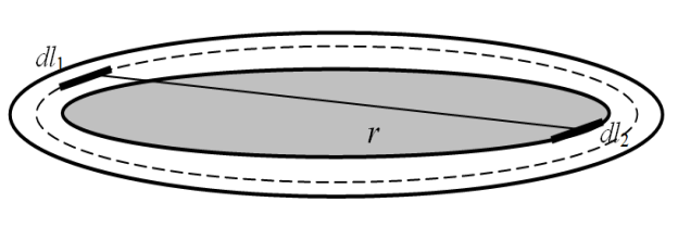
Grey surface crossed by the external flux.

Field intensity inside a cylindrical conductor (Напряжённость поля внутри цилиндрического проводника)

I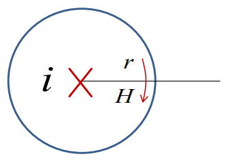 nfinitely long cylindrical wire with the radius of R, and the current of i.

The field intensity inside the conductor at the point with the radius of r satisfies the Ampere Law.

- current which crosses chosen contour.

Directions of the intensity vector and vector are the same.

This integral may be replaced by:

Current density:

Field intensity:

Flux linkage of a thin current layer (Потокосцепление тонкого слоя с током)

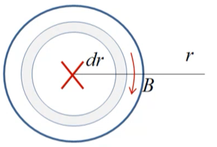
Consider a thin cylinder with the radius of r and the thickness of dr

T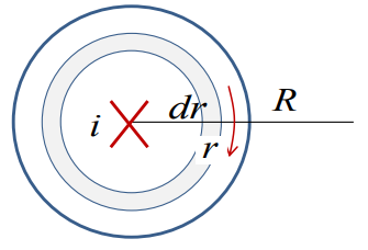 he current inside this layer is:

The flux per unit length:

In principle we assume that somewhere there should be wire with the opposite current.

After integration:

The flux linkage of a thin layer:

Total internal flux linkage:

or:

Internal inductance of a thin conductor (Внутренняя индуктивность тонкого проводника)

Transformation of the last integral:

Taking into account the limits:

Final expression:

Internal inductance:

External inductance of two-wire transmission line (Внешняя индуктивность двухпроводной линии)

F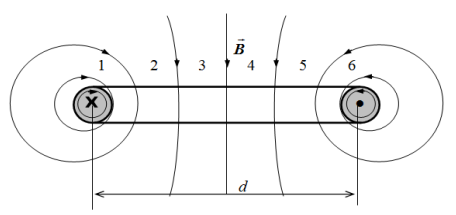 lux density induced by a wire:

External flux:

R – radius of the wire; R<<d

Similar flux induced be the second wire.

The total external flux:

Flux linkage:

Inductance:

Internal inductance:

External inductance:

Лекция 4. Method of images (метод зеркальных изображений)

Image method for the flat boundary between dielectrics (метод изображения для плоской границы между диэлектриками)

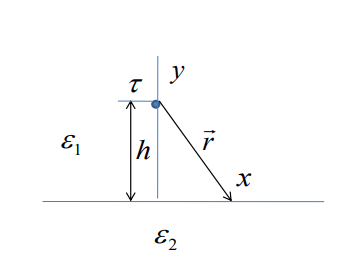
Application of the image method is not so evident. Look at this picture. Here the electric field exists in both half-spaces. Each half-space requires separate solution. We can notice this flat surface. It is this horizontal line. This dot corresponds to a charged line. Infinitely long charged line with the linear charge density τ. This charged line suspended above this surface at the high h. This surface is really an interface between two dielectrics with different properties. Above this surface the dielectric permittivity is equal to ε₁ below the dielectric permittivity is equal to ε₂. Find the field intensity distribution everywhere in the space in both sub-spaces (above the interface and below the interface (граница раздела)).

The electrostatic problem is described by the Poisson and Laplace equations. This equation has a unique solution in the case when we have defined proper boundary conditions. This may be definition of the potential at the border of the considered space; or normal derivative of the electric potential or intensity of the electric field because the normal derivative of the potential is really the normal component of the electric field intensity or if the medium has the constant dielectric permittivity, then it is identical to the case when we shall define a normal component of the field displacement.

- field induced by charged line source. This expression works only in the case when there are no surfaces. There is only one space with one dielectric permittivity is everywhere the same.

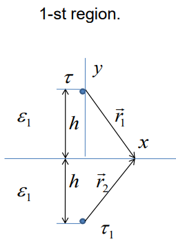
Let's suppose that the electric field in the upper half-space above the interface may be calculated as the superposition of two electric field. The first of them induced by initial wire itself, by the primary source. However, there will be also a component, which is induced by another wire. The wire, which is placed under the surface and which has a charge density ₁.

Dielectric constant is the same in both half-spaces ε₁. Let us place the image into the point of . Charge density of the image is .

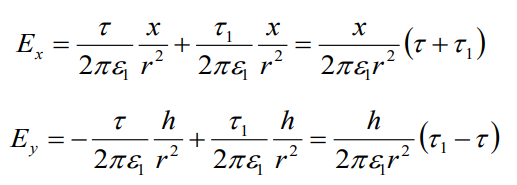
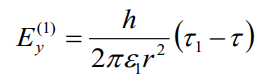
Field intensity in the boundaries:

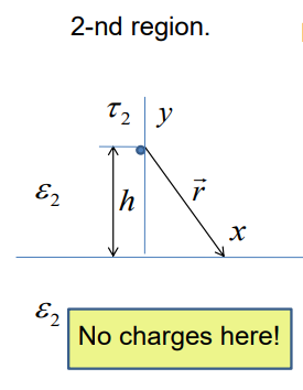
Let’s suppose that the dielectric permittivity of the hole space is ε₂. Now there should not be any charge in the lower space. But above the surface there will be a charge with unknown density . This charge, which is placed above the surface at the distance h.

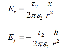
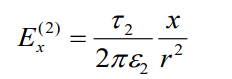
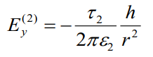
Field intensity at the boundaries:

Boundary conditions are:

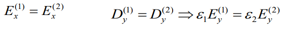
In the upper half-space

In the lower half-space

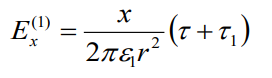
First relation or

Boundary conditions for vertical component of the field intensity

In the upper half-space

In the lower half-space

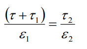
Second relation:

Combining with the first relation: or

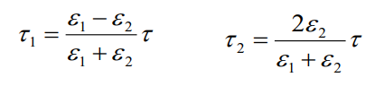
If the boundary conditions are satisfied then the solution is unique one. There are no other solutions. That is why such mirror reflection is the only one possible.