Transmission of energy in a dc line (Передача энергии в линиях постоянного тока)

Similar consideration may be made for the load which consists of resistor, capacitor, and inductance. We should simply split the total energy which crosses this surface into several parts.

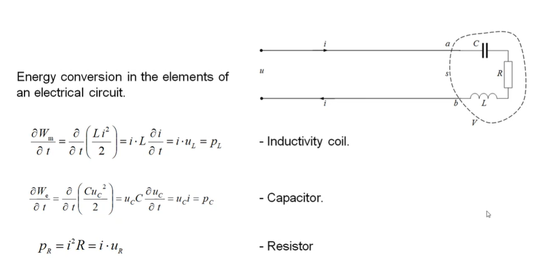
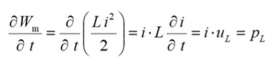
First of them, ∂W_m/∂t, the energy of the magnetic field which crosses this area corresponds to the magnetic field which is induced by inductance and is equal to

.

In any time moment, this power should not be equal to zero, but if the inductivity coil is ideal, of course, this power integrated, for example, by period will be equal to zero in any case.

A similar consideration can be done for the capacitor. Finally, we shall come to the same conclusion – it’s equal to the power which correspond to the capacitor.

And from the previous consideration we can also conclude that power in the resistor which is dissipated here is equal to such a product.

Now, this energy comes to the load from the external electromagnetic field and may be expressed as integral over the surface from E cross H, ds.

It is ∂W/∂t and then plus the energy which is dissipated in resistors. The energy ∂W/∂t is dependence of the energy stored in the inductance and capacitor and it is equal i·u_L+i·u_C and also i·u_R. We can transform this to i times sum of these voltages. It is power. Again, we can find out that energy that crosses this area is equal to the power, which now is not dissipation of the energy but the power of the energy transformation (into the heat, electric field, magnetic field). The power of the flow of electromagnetic energy entering the surface S is equal to the total power consumed in the circuit between ab terminals.

The field picture near the wires with current (Картина поля вблизи провода с током)

That’s the general picture which corresponds to the transmission line with arbitrary load. Due to the presence of a small tangential component of the electric field strength vector at the surface of the conductor with current, the resulting electric field strength vector E is not perpendicular to the surface of the conductor. This leads to the appearance of the normal component of the Poynting vector at the surface of the conductor. Consequently part of the transmitted energy is absorb inside the wires of the transmission line.

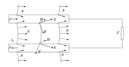
There are two wires which carry current to the load and from the load. Certainly, there should be a voltage between these two wires that’s why that’s a line which shows the electric field in the space around these wires. The normal component of the electric field corresponds to the voltage between wires that’s the voltage as if two lines form a capacitor. But also, there is a horizontal component which corresponds to the Ohm's Law, in such a case the Poynting’s vector will come just inside the wire, partly, the energy is transformed from the source to the load, and the horizontal part of the Poynting’s vector just illustrate this energy, transformed from the source to the load. But the small vertical component of the Poynting’s vector illustrates the power, which is dissipated in non-ideal wires. If the wires are ideal than there should not be component of the Poynting’s vector which will come inside the wire. All these S-vectors will be parallel to the wire surface. H here in any case is induced by the current inside wire and the H-field, magnetic field, circulates around the wires, H-vector has no component which is directed from the power source to the load, this vector is always normal to our surface.