The momentum of the electromagnetic field (Момент электромагнитного поля)

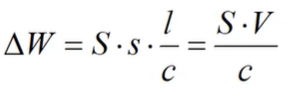
Delta W, this is the energy that crosses some area is equal to S, Poynting vector, times V, a volume of this cylinder, over the c, velocity of the light. Now the important relation between the energy and mass. If some area was crossed by energy ΔW, we can say that the same area was crossed by the mass with respect of relation

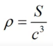
That’s a formula that was written by Einstein initially, energy is equal to m times c squared, the universal relation which is valid in any kind of situation. Delta W is delta, c is constant so delta can be implied only to the mass. Delta m is the mass, which is concentrated inside this consider cylinder. So, the electromagnetic matter has some equivalent density:

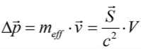
Here the impulse that is traditionally equals to mass times velocity, and it is equal S over c squared times the volume, which is occupied by the material in this matter.

And coming back to our problem. What we have considered is right for the horizontal cylinder, where the matter passes along the same line, in our case the situation is different because the electromagnetic material travels along different trajectories. That’s why we have to integrate this relations over the volume.

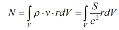
This matter which circulates around the central axis creates the angular momentum (момент количества движения) that is equal to radius times mass times v. According to relation that was found for the density of the electromagnetic matter, we shall get such an expression. Taking into account the Poynting's vector

,

and the element of volume is 2π·r·dr, we can find an angular momentum. Strange situaion, let’s assume we shall switch off for example magnetic field, it is absolutly static situation, there is capacitor with electric field inside, but in the nature there is a law of the conservation of the angular momentum, the magnetic field will dissapear, it is possible to achieve, but what is impossible to change without consequences - the angular momentum, we can’t do this, nature forbid that. What is that mean? If we shall remove the edge, the magnetic field, than the cylinder will start to rotate itself. Or another approach – we shall switch off the electric field, discharge this capacitor, in such a case again the angular momentum of the electromagnetic matter will be come to be equal to zero but the law of the conservation of the angular momentum means that in this case the cylindrical capacitor will start to rotate. It was prooved that electromagnetic field, matter really has it's mass.

Лекция 8. Numerical Methods of the Electromagnetic Field Modeling. (Численные методы моделирования электромагнитного поля) Classification of the numerical methods (Классификация численных методов)

There are two different items, that are used for this classification. First of them, evidently the use the method depends strongly on the problem, which it solves. That is why first classification is classification of the problems.

Classification of the problems (Классификация проблем)

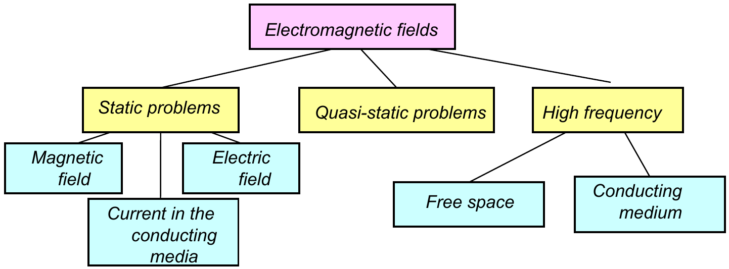
• Static problems – do not depend on time (DC current in the conducting media). This problem is differing from the electrostatics. We already define what is it electrostatics. First property of this field is absenting of the time dependent fields and there are no currents. So, really these three different types of the problem.

• Quasi-static problems – usually here assumed the electromagnetic field which changing time according to sinusoidal dependence. But it isn’t exactly so. This type of electromagnetic problems covers also transient processes (переходные процессы). But the main property of this type of problems is that we neglect one part of the currents – displacement current. Usually this corresponds to low frequency or the transient processes with small rate of the electric or magnetic field components time dependence. In such a case, we first consider interaction between the electric field and magnetic field inside conductors.

• High frequency – usually these high frequencies are considered in free space. That corresponds for radio waves, for example. But also, sometimes high frequencies fields are considered in the conducting medium. Typically, this is not the case which is considered by high frequency problems because the current in the conductors assumes, that there are no displacement currents because displacement currents by default are not introduced in conductors, but in the case of bad insulator (material is in insulator, but there is a very small conductivity. So, the conductivity currents may influence on the final balance between electric and magnetic field.). In such not very often mad (?) cases a nevertheless high frequency equations are implemented to calculate the electromagnetic field inside these bad conductors.

So that is the general overview of the problems which may be solved both analytical methods, if the geometry of the system is simple enough or in general cases by numerical methods.