General solution of the Laplace’s equation in a cylindrical coordinate system (Общее решение уравнения Лапласа в цилиндрической системе координат)

Combining the solutions, we will get:

This function is known as circular (angular) harmonic of order k.

General solution:

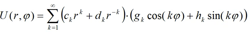
c_k, d_k, g_k, h_k – these coefficients correspond to different numbers (different harmonics) of the order of k.

Application of the variable separation method for the magnetic field modeling (Применение метода разделения переменных для моделирования магнитного поля)

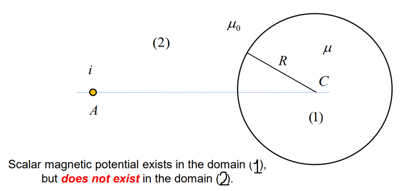
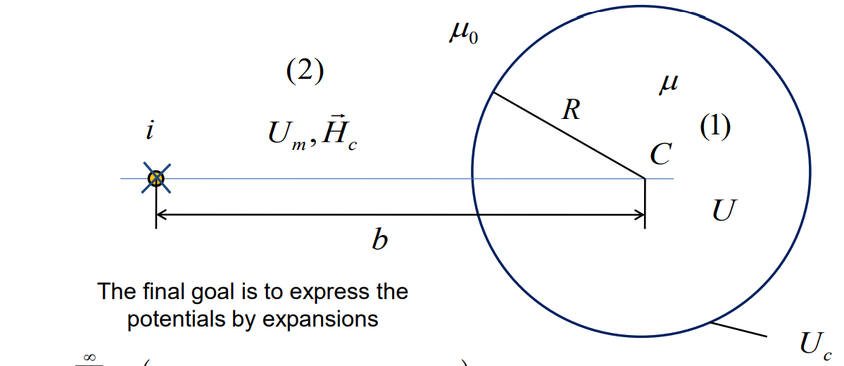
We have a wire with the current and in any case the scalar magnetic potential can’t be used to describe the magnetic field inside the wire. Let’s split our domain in two parts: (1) – the inner part of the cylinder; (2) – everything, which is placed outside the cylinder. (1) – no currents, so we certainly can describe the magnetic field in terms of scalar magnetic potential. We can’t use the scalar magnetic potential in (2), because it doesn’t exist.

Reduced scalar magnetic potential (Редуцированный скалярный магнитный потенциал)

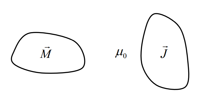
The left domain – ferromagnetic; and the volume (right), where currents induce the magnetic field in the whole space.

Magnetic field intensity may be presented as:

is the field intensity induced by the current sources

is the field intensity induced by the magnetized objects

Our problem is linear. It means that μ doesn’t depend on the value of magnetic field intensity, but this principle of superposition is correct for any kind of magnetic system, doesn’t matter isn’t linear or not.

is the potential field:

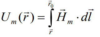
A special potential may be introduced:

Combination of scalar magnetic potential and reduced magnetic potential (Комбинация скалярного магнитного потенциала и редуцированного магнитного потенциала)

Reduced magnetic potential exists in the whole space Scalar magnetic potential exists only in a simply connected domain with no currents inside

We should use total magnetic scalar potential inside the magnetized object and everywhere else outside the magnetized object, we can use another presentation of the magnetic field.

Inside the - domain: , U is the scalar magnetic potential

Outside the - domain:

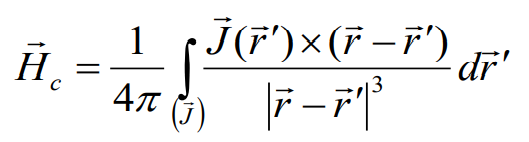
The field induced by current sources may be calculated by Biot – Savart Law:

Domain (1) – magnetized object is described by the Laplace equation.

Inside the magnetized domain (1) the scalar magnetic potential satisfies the differential equation

(1): if   const

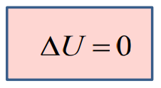
In (2) everywhere  = ₀ = const, that’s why the potential satisfies the Laplace equation.

In the domain (2) the reduced magnetic potential satisfies the differential equation

(2): This equation is valid in the domain (1) as well.

Both equations are the same but the variables are different

 – is the border of the domain with the magnetized matter Inside the magnetized domain: Scalar magnetic potential of the currents:

Solution of the problem should provide boundary conditions on 

(tangential components of the magnetic field are the same at both sides of this border)

may be calculated as a gradient of the total magnetic potential inside the 1^st domain.

We can consider the magnetic field as a superposition of these two components:

or:

, - reduced magnetic potential; – the potential, which is induced by currents (but the currents can’t be described by the scalar magnetic potential. We consider the field which is induced by the currents only along the surface , but there are no currents along this surface. That’s why in principle we also can use such an item as scalar magnetic potential induced by currents.) Of course, this equality also depends on the choice of points of zero potentials, so it is necessary to choose properly points with zero potentials. Otherwise, there should be added some uncertain constant, because potential is defined only with respect to the uncertain constant.

From the condition for the normal components, we can easily come to the relation for the normal components of the field intensity.

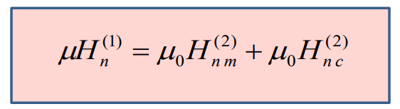
We can use this relation exactly for the magnetic field intensity. It is valid independently on how we defined the magnetic potentials.

Magnetic field of the line current near a magnetized cylinder (Магнитное поле линейного тока вблизи намагниченного цилиндра)

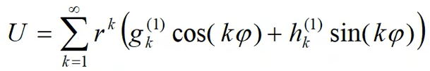
- general solution The origin of the coordinate system in point C. If we use a general form of solution, we should substitute radius with the zero value. In such case the potential will be infinitely big. To avoid this infinity, we need to assume that the coefficient at the term of 1/r will be always equal zero. Otherwise, the expression of the potential simply will not exist (в итоге получаем такую шнягу ↓, тут он объясняет, почему правая часть выражения преобразовалась)

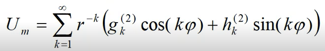
Similar situation is with the presentation of the solution for the reduced magnetic potential. The radius may be infinitely big. That doesn’t destroy the solution because this will be one over infinitely big value in any power =0. But the r = 0 is excluded from the domain (2). That’s why this term will be never infinitely big.

We should somehow define the constants (g⁽¹⁾_k, h⁽¹⁾_k, g⁽²⁾_k, h⁽²⁾_k). First of all, we will start with the question: where the potential is equal to zero. We can choose this point everywhere. But we choose the point with zero potential just at this horizontal line (b). It’s the most convenient choice. But why? Let’s look at general structure of the magnetic field here. We have already known that field along the line will have only a vertical component (see mirror images). So, we can integrate Hdl over the line (b), Hdl – scalar product. We always have zero answer. That’s why all potentials at this line are the same and it’s convenient to choose them to be equal to zero. We will use this choice later to decrease number of unknown coefficients.