

First type boundary conditions (Первый тип граничных условий)
Let’s assume we know 1-st type boundary conditions.
![]()
What does that mean? We know potential distribution over the boundary, so we simply do not need to solve this equation in the boundary nodes, because we already know the solution, that’s why this second term, which includes the integral over the whole boundary is not used at all.
![]()
It is not necessary for the nodes which are placed inside the problem domain, and we already know the solution for all external nodes. That’s a lucky situation and so we completely got view of this second term. In principle, sometimes when we work with the second type boundary conditions the situation is more complicated. The 1-st type boundary conditions keep a symmetry of the main problem matrix.
The potential and field intensity (Потенциал и напряжённость поля)
What should we do after we have found the potential solving the problem, which is based on Galerkin method? We have found an approximation of the potential over the whole problem domain, node only inside the certain triangle, it is now described by such a sum:
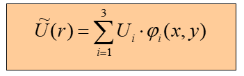
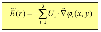
So, if we need field intensity we can apply the gradient operator, and this gradient operator will give us such expression for field intensity everywhere in the problem domain, not only in one triangle, as we discuss before.
2-nd type boundary conditions (Второй тип граничных условий)
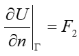
2-nd type boundary conditions assume the normal derivative of the potential is equal to some function.
And we have here an integral along the boundary and we can substitute the boundary conditions of the second type inside this relation and we shall get a final result.

The equation for the external nodes, which are placed at the boundary, are more complex. The exception corresponds to the case when this function F2 is equal to zero, in such a case the form of the coefficients will be identical because this derivative is equal to zero the first integral in the right part also will be equal to zero. The 2-nd type boundary conditions of the dU/dn = 0 is most often used boundary condition, so in such a case if we have such a situation than we can say the expression for the coefficients within the finite element method is always the same and it is described by these simple relations.