Лекции_Микроэкономика

A.Friedman ICEF-2012

Proof. Let firm 1 is located by distance a from the left corner and firm 2 by distance b from

function with respect to a and b we get the following first order conditions

a 1 a b 0.5 01 a b 0.5 b 0 .

Solving this system we get a b 1/ 4 .

91

7. FACTOR MARKETS (in the new syllabus there is no separate topic: demand is studied in the theory of firm and supply - in consumer theory)

7.1 Demand for factors

We get individual firm’s demand by solving its profit maximization problem

max TR Q K ,L TC K ,L

K 0,L 0

That is marginal revenue product of a factor (MRP) should be equal to the marginal factor cost (MFC).

If output market is perfectly competitive, then MR p and MRPi pMPi .

If factor i market is competitive, then MFCi TC x wi .xi

Thus, if all (input and output) markets are perfectly competitive, then factor demands can be found from the solution of the system pMPi wi .

Consider two-factors model. Assuming diminishing marginal product of each factor and fixing the amount of capital used the value of marginal product of labour gives the inverse labour demand curve

w

w

pMPL K

Firms’ demand curve for a factor and industry demand curve.

To get industry demand curve for a factor (in case of perfectly competitive industry) we should take into account the product-price effect.

To simplify analysis let us assume that labour is the only factor of production. As individual firm demand for an input is given by its MRP curve, then we should sum up individual demand by taking the horizontal sum of MRP curves. But the resulting curve does not correspond to industry demand. Suppose initially industry economy was in equilibrium with output price p0 , input price w0 and market labour demand L0 . If wage rate falls, then each

firm will demand more labour and we move to L . But as employment goes up the quantity

92

only till L1 . This analysis suggests that the industry supply curve is steeper (less price elastic) than the horizontal sum of the firms’ demand curves.

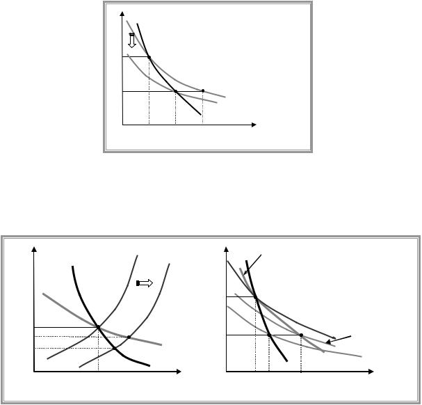
Conclusion 1. The lower elasticity of demand for the product, the lower the elasticity of demand for a factor.

Explanation. With more price elastic demand for final product (flatter output demand curve) the price fall would be smaller and a result downward shift of the MRP sum would be less, which results in larger employment and flatter (more price elastic industry factor demand).

Firms’ demand curve for a factor in the SR and in the LR

In the short run capital is fixed and MRPL K0 gives the firm’s demand for labour. But in the LR capital adjusts and a s a result MRPL curve shifts.

Two inputs are said to be complementary (anticomplementary) if increased use of one input raises (reduces) the marginal product of the other. If one input has no effect on the marginal product of the other input, then factors are said to be independent.

Let initially at w w0 firm’s long run demand is given by L0 ,K0 . Suppose wage rate falls till w1 w0 . In the SR firm will demand more labour, which can be illustrated by movement to the right along the SR demand.

If factors are not independent, then MPK would be affected and capital will adjust in the LR, which in its turn would affect the position of MRPL curve. Here two cases should be considered separately.

93

A.Friedman ICEF-2012

(a) K and L are complementary.

As labour increases in the SR, then marginal product of capital increases and as a result

MRPL K1 MRPL K0 ). As marginal productivity of labour goes up firm finds profitable to use more labour, thus in the LR labour increases more than in the SR

(b) K and L are anticomplementary.

As labour increases in the SR, then marginal product of capital falls and as a result MRPK r

. Thus firm will use less capital, that is K1 K0 . As a result marginal product of labour goes up and brings an upward shift of MRPL curve (since MRPL K1 MRPL K0 ). As marginal

productivity of labour goes up firm finds profitable to use more labour, thus in the LR labour increases more than in the SR

Summary: demand curve is flatter (more price elastic) in the LR than in the SR.

Conclusion 2. Given either complementarity or anticomplementarity between inputs, the demand curve for an input is flatter (more price elastic) in the LR than in the SR (when some factors are fixed).

Conclusion 3. Factor demand curves always have negative slope (i.e. there is no such thing as a “Giffen factor”.

Analytical proof. Let firm uses two factors of production L,K , with corresponding prices w and r . Let us fix the output price p and consider two different vectors of factors prices

under given prices, then any other combination of factors can not result in higher profit and similarly for ( L0 ,K 0 ) :

pf ( L ,K ) w L rK pf ( L0 ,K 0 ) w L0 rK 0 pf ( L0 ,K 0 ) w0 L0 rK 0 pf ( L ,K ) w0 L rK .

Adding up these inequalities we get:

w L w0 L0 w L0 w0 L or 0 w ( L L0 ) w0 ( L L0 ) ( w w0 )( L L0 ).

94

labour either fall or stay the same: L L0 .

The difference with consumer theory: when price of a factor goes up initial combination of factors is still affordable for the producer as he does not face with financial constraint.

Demand for a factor and supply of other factors.

To simplify the analysis let us assume that product-price effect is negligible.

Let initially industry was in the long-run equilibrium with w0 , r0 and factors employment of L0 and K 0 . Suppose that wage rate falls till w1 w0 . In the SR industry labour employment goes up from L0 to L1SR .

If factors are not independent, then MPK would be affected and capital will adjust in the LR,

which in its turn would affect the position of industry labour demand curve. Here two cases should be considered separately.

(a) K and L are complementary.

As labour increases in the SR, then marginal product of capital increases and as a result MRPK r . Thus demand for capital goes up, which results in an increase in capital employment: K1 K0 . As a result marginal product of labour goes up and brings an upward shift of MRPL curve for each firm (since MRPL K1 MRPL K0 ). As marginal productivity of labour goes up each firm will use more labour and industry demand curve shifts to the right. Finally labour increases from L0 to L1LR .

(b) K and L are anticomplementary: result is the same in terms of labour but K1 K0 (FOR SELF-STUDY).

Let us analyze the role of elasticity of capital supply curve. With flatter (more price elastic supply of other factor) its employment will change more in response to increased demand, which results in greater shift in the SR labour demand curve. As a result LR industry demand for labour would be flatter (more price elastic).

Conclusion 4. An industry demand for a factor is less elastic the less elastic is the supply of other factors.

95

7.2 The supply of factors and competitive equilibrium

Individual supply curves could be derived from consumer’s utility maximisation problem (it was studied in the theory of consumption).

Although individual labour supply could be backward bending the market supply curve is likely to be upward sloping. Explanation: even if some workers that are currently in the industry may prefer to work fewer hours as the wage rises, new workers will be attracted (from other industries or from leisure).

Elasticity of supply of a factor to a particular use depends

on the degree of specificity of the factor to this use?

on the length of time allowed for the factor to be reallocated to or away from that use.

Factor market equilibrium.

w

L L

Input earnings can be divided into two components: transfer earnings and economic rent.

Transfer earnings are the amount that any unit of a factor must earn in order to prevent it from transferring to another use.

Economic rent is any excess over transfer earnings that a unit actually earns.

Factor payments which are economic rent in the SR and transfer earnings in the LR are called quasi-rents.

7.3 Monopsony and monopoly in factor markets

Monopoly on the supply side of the input market.

By combining into a trade union workers (with no market power individually) may by collectively restricting the supply of labour, raise their wages.

Examples of trade union objectives:

(i)the rent maximization,

(ii)the total wage bill maximization.

Consider labour market with linear demand curve for labor LD A bw and linear labour

supply curve: LS cw , where A c . Suppose that labor market is controlled by monopolistic labour union that maximizes economic rent.

Economic rent is any excess over transfer earnings that a unit actually earns

96

w0

98

8. GENERAL EQUILIBRIUM AND WELFARE ECONOMICS

8.1 Pareto efficiency

Ana allocation is feasible if consumption of each commodity equals to the amount available in the economy.

A feasible allocation of resources is Pareto optimal (efficient) if there is no other feasible allocation that will make some person better off without making anyone else worse off.

Pareto improvement is a reallocation of resources that makes at least one person better off without making anyone else worse off.

Any interior Pareto efficient allocation has to satisfy the following efficiency conditions:

Efficiency in consumption,

Efficiency in production,

Efficiency in output mix.

Consider an economy with two consumption goods ( X ,Y ), two factors of production ( L,K ) in fixed supply and two individuals ( A,B ).

Efficiency in consumption

An allocation of commodities is efficient in consumption if given the total amount of each commodity available for consumption, the only way to make one person better off is to make another person worse off.

Thus we assume that supply of each commodity is fixed and deal with exchange economy. Feasible allocations in exchange economy can be illustrated graphically by Edgeworth box.

Y A

X

Assume that both agents have well behaved preferences. Their preferences can be illustrated in the Edgeworth box by indifference curves.

99

Increase in A

utility

Y

Increase in utility of agent В

O A X A

X Y B

Consider allocation C. It is not efficient in consumption since both persons would be better

Preferred by A

possible. As agent A values good X more relative to agent B, we should reallocate good X in favour of agent A. Suppose we take small unit of good X from B and give it to A. Then A is willing to scarifies up to units of good Y. Let us take only ( ) / 2 units of good Y from

agent A. As a result he would be better off as ( ) / 2 . If we give ( ) / 2 units of good Y to agent B, he would be better off as well since he would be as well off by getting units of good Y instead of one unit of X but gets more ( ) / 2 . Thus by reallocating

of resources we were able to improve the position of both agents, which means that initial allocation was not Pareto efficient.

100