

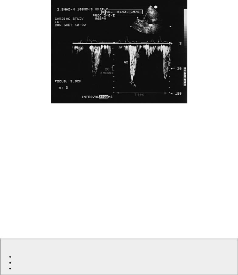
Figure 1.3 Doppler images display flow velocities on the vertical axis and time on the horizontal axis. Blood flow for specified areas in the heart is seen as it accelerates, reaches a maximum velocity, and then decelerates throughout the cardiac cycle. This CW Doppler tracing of aortic flow (AO) in a dog has a velocity of 143 cm/sec (A).
This chapter deals with the physical principles of sound waves that allow ultrasound to be used as a diagnostic tool. The physics of ultrasound involves an understanding of the basic properties of sound waves and how these properties affect transducer selection, image quality, and diagnostic interpretation. Only the principles needed to make knowledgeable technical decisions and diagnostic interpretations are presented in this chapter. More detailed information can be found in books dedicated to the physics of diagnostic ultrasound. Selected references are listed at the end of the chapter.
Basic Physics
Cycles and Wavelengths
Sound waves travel in longitudinal lines within a medium. The molecules along that longitudinal course of movement are alternately compressed (molecules move closer together) and rarefacted (molecules are spread apart). The time required for one complete compression and rarefaction to occur is one cycle (Figure 1.4). The distance in millimeters that the sound wave travels during one cycle is its wavelength.
Sound Waves
Alternately compress and spread apart the molecules in their pathway. 1 cycle = one complete compression and expansion
Wavelength = the distance traveled during 1 cycle
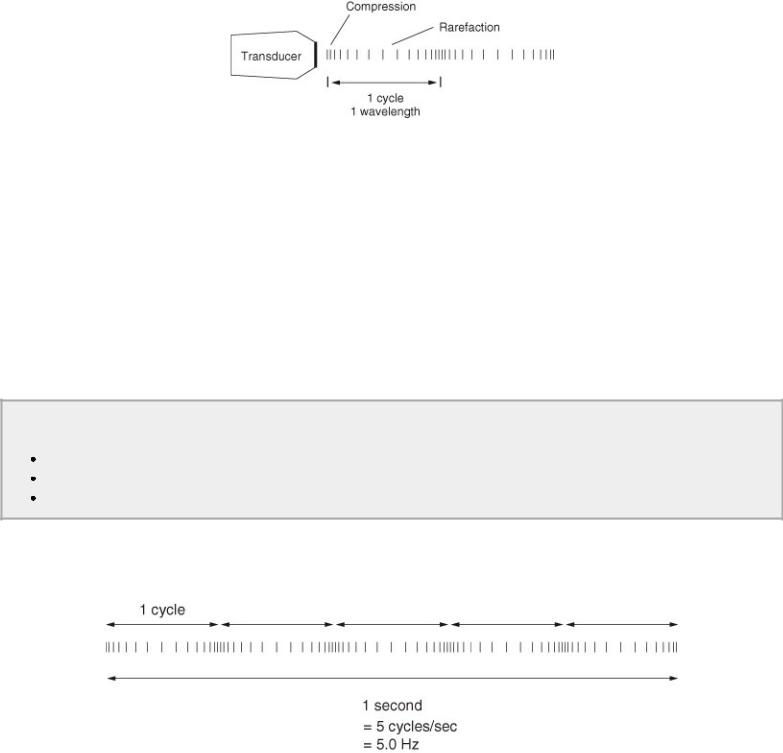
Figure 1.4 Sound waves cause compression and rarefaction of the molecules along their path. The time for one complete compression and rarefaction to occur is called a cycle. The distance sound travels during one cycle is measured in millimeters and is its wavelength.
The source of the sound wave determines the length of a cycle. Transducers generate the sound in diagnostic ultrasound. They will be discussed in detail later, but for any given transducer the wavelength is constant.
Frequency
The number of cycles per second is the frequency of the sound wave (Figure 1.5). Frequency is measured in Hertz (Hz), where 1 Hz equals one cycle per second. Ultrasound has a frequency greater than 20,000 cycles per second, and is beyond the range of human hearing. Since frequency is the number of complete cycles per second, the higher the frequency of the sound wave the shorter the wavelength must be.
Frequency
The number of cycles per second = frequency
High frequency = shorter wavelengths
Low frequency = longer wavelengths
Figure 1.5 The number of cycles per second is the frequency of the sound wave. Frequency is measured in Hertz (Hz). One Hz equals one cycle per second.
A 5.0-megahertz (MHz) transducer transmits 5 million cycles per second at 0.31 millimeters (mm) per cycle, while a 2.0-MHz transducer transmits only 2 million cycles per second at 0.77 mm per cycle. Table 1.1 lists wavelengths for sound generated at various frequencies.
Table 1.1 Wavelength of Sound at Commonly Used Frequencies
Frequency (MHz) |
Wavelength (mm) |
|
|
2.0 |
.77 |
|
|
3.5 |
.44 |
|
|
|
|
5.0 |
.31 |
7.5 |
.21 |
|
|
Speed of Sound
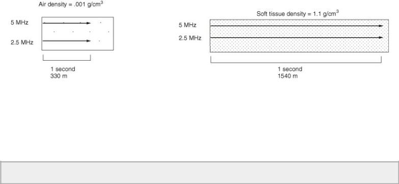
The speed of sound (V) depends upon the density and stiffness of the medium through which it is traveling. Increased density allows sound to travel faster. The velocity of sound does not change within a homogeneous substance and is independent of frequency (Figure 1.6). Table 1.2 lists the speed of sound in various tissues. The speed of sound through air is very slow because of its low density, while bone allows sound to travel at relatively high speeds.
Table 1.2 The Speed of Sound in Soft Tissues
Tissue |
Speed(m/sec) |
|
|
air |
330 |
|
|
fat |
1,440 |
|
|
brain |
1,510 |
|
|
liver |
1,560 |
|
|
kidney |
1,560 |
|
|
muscle |
1,570 |
|
|
blood |
1,570 |
|
|
bone |
4,080 |
|
|
Figure 1.6 Increased tissue density allows sound to travel faster. Sound generated by a 2.5-MHz transducer and a 5.0-MHz transducer will have the same velocity within the same tissues since the speed of sound is not affected by frequency.
The average velocity of a sound wave in soft tissue is 1,540 meters per second regardless of transducer frequency (Figure 1.7). Velocity is calibrated into the ultrasound machine, which then calculates the distance (D) to cardiac structures based upon how long it takes to receive reflected echoes (T):
Equation 1.1 
Transducer frequency does not affect the speed of sound in tissues.
Figure 1.7 Sound travels through soft tissues at an average velocity of 1,540 m/sec regardless of transducer frequency. The time required to travel 1 cm at 1,540 m/sec is 6.5 microseconds (µsec) one way and 13 µsec round trip.
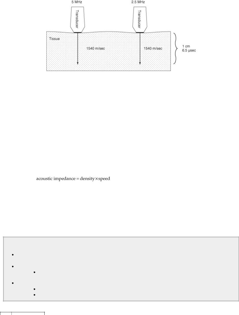
The time (T) required to travel 1 cm is 6.5 microseconds or 13 microseconds round trip. Even though sound must travel through various tissues with slightly different velocities during an echocardiographic exam, the equipment is calibrated for the average speed of sound in soft tissues (1,540 meters per second). Structures are displayed on a monitor at the calculated depth, and an image of the heart is created. This always creates some degree of error in calculating true structure depth, but the error is generally negligible.
Acoustic Impedance
Acoustic impedance is the opposition or resistance to the flow of sound through a medium. Impedance depends upon the density and stiffness of the medium and is independent of frequency. Very stiff or hard materials are hard to compress and rarefact. Therefore, although increased density increases the speed of sound, if the ability to compress and rarefact a sound wave is limited, the impedance or resistance to sound transmission is high.
Equation 1.2
Contradictory as it sounds, the higher the density and the greater the velocity of sound through a medium, the greater the resistance is to sound transmission. Table 1.3 lists the acoustical impedance of sound in various tissues. Because of its stiffness and inability to compress and rarefact molecules easily, bone has high impedance, while air, because its molecules are easily compressed and rarefacted, has low impedance. High acoustical impedance is what produces a high degree of sound reflection at bony or air interfaces, creating a shadow on the ultrasound image beyond the bone or air due to lack of further sound transmission.
Reflection of Sound
Depends upon acoustical mismatch
 The greater the difference in acoustical properties the greater the degree of reflection. Depends upon angle of incidence
Sound striking an organ perpendicularly will have a large amount of sound reflected straight back to the transducer.
Depends upon reflecting structure’s size
Must be at least 1/4 size of the wavelength
Higher frequency transducers can reflect sound from smaller structures.
Table 1.3 Acoustical Impedance of Various Tissues
Tissue |
Impedance (g/cm2 sec) |
bone |
7.80 × 10⁵ |
muscle |
1.70 × 10⁵ |
kidney |
1.62 × 10⁵ |
blood |
1.61 × 10⁵ |
brain |
1.58 × 10⁵ |
fat |
1.38 × 10⁵ |
air |
.0004 × 105 |
Reflection, Refraction, and Scattering
Reflection is sound that is turned back at a boundary within a medium. These reflected echoes are called specular echoes. When an interface between two tissues with different acoustical impedances is reached, a portion of the sound is reflected back to the transducer. The rest continues on through the tissues. The greater the difference in acoustical impedance the greater the degree of reflection. For the same reason, if two boundaries have little or no acoustical mismatch they will not be identified as two different tissues. Therefore interfaces between muscle and fluid, as in the heart, will reflect sound at different intensities while the cells within the homogeneous muscle itself will reflect sound with similar strengths.
All interfaces between muscle and blood-filled chambers in the heart have slightly brighter boundaries on the ultrasound image because of this increased reflection. The interface between tissue and air has an even greater difference in acoustical impedance, and therefore the pericardial sac around the heart is always one of the brightest structures on the ultrasound image. The gel placed between the transducer and skin surface is used to prevent the large degree of reflection ordinarily seen between a tissue and air interface.
The angle at which sound strikes the reflective surface (the angle of incidence) determines the angle of reflection. The angle of reflection is equal to the angle of incidence (Figure 1.8). When sound is directed perpendicular to a structure the angle of incidence is zero and the sound is reflected straight back to the transducer. If the angle of incidence is 50°, then the angle of reflection will also be 50°. When the angle of incidence is 90° or parallel to the interface, no sound will be reflected back to the source. This principle tells us that the best two-dimensional and M-mode cardiac images are obtained when sound is directed perpendicular to the tissues.
Figure 1.8 The angle of reflection is equal to the angle at which sound strikes the tissue. Sound that is directed perpendicular to the tissue is reflected straight back to the transducer producing the best images. Sound is refracted when it crosses a boundary between two different tissues. The greater the difference in acoustical properties between the two tissues, the greater the degree of refraction.
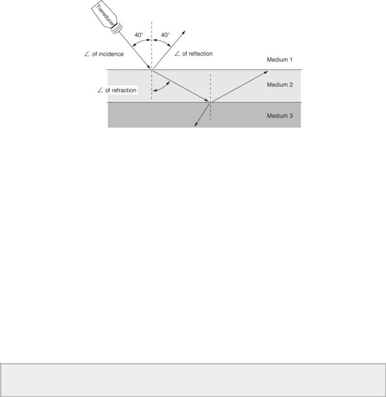
Not all sound is reflected however, and some continues on through the tissues. These sound waves are refracted if the two tissues are different (Figure 1.8). Refraction is the change in direction of sound as it travels from one medium to another. This is similar to what happens when light waves in water create a distorted image. The greater the mismatch in acoustical impedance between the two tissues the greater the degree of refraction. As the refracted sound beam travels in a new direction, the angle of reflection with respect to the original source is different, and positional errors can result since the transducer thinks the received sound is coming from the same direction as the sound waves it generated earlier.
The errors produced by refraction during an examination create few problems unless the refracted beam has to travel a great distance. An angle of 1 or 2 degrees at the top of the refracting tissue can result in a several millimeter error in position by the time it reaches the far side of a deep structure. When the two mediums differ enough to create a refractive angle of greater than 90° (as with soft tissue and bone) then an image is not generated beyond the second structure.
Reflection of sound is not only dependent upon the acoustical mismatch of two tissues but also upon the structure’s size. The structure must be at least one-quarter the size of the wavelength for reflection to occur. The short 0.21-mm wavelengths of a 7.5-MHz transducer are reflected from structures that are as small as 0.05 mm in thickness, while structures must be at least 0.19-mm thick for the 0.77-mm wavelengths of a 2.0-MHz transducer to be reflected. High frequency transducers then, provide higher resolution images since smaller structures reflect their sound waves.
↑ Frequency = ↓ Wavelength = ↑ Resolution
↓ Frequency = ↑ Wavelength = ↓ Resolution
Structures that are small and irregular with respect to the sound wave do not reflect sound but rather scatter it in all directions without regard for the angle of incidence (Figure 1.9). Some of this scattered sound is directed back to the sound source and is what allows ultrasound to give us information about tissue character. Scattered sound is important for the generation of images from objects with large angles of incidence to the sound beam or small structure-like cells.
Figure 1.9 Structures that are small and irregular with respect to the wavelength cause sound to be scattered in all directions. Some of this scattered sound will be directed back to the transducer for image generation. Scattered sound is important in tissue characterization.
Attenuation
Sound traveling through a medium is weakened by reflection, refraction, scattering, and absorption of heat by the tissues. This loss of energy is called attenuation. High frequency sound attenuates to a greater degree than lower frequency sound because its wavelength allows it to interact with more structures. This is the reason the deep bass sounds of an orchestra carry farther than the high-pitched sounds. The large degree of attenuation with high frequency sound leaves less energy available for continued transmission through the medium.
↑ Frequency = ↓ Depth
↓ Frequency = ↑ Depth
The half-power distance of a tissue is the distance sound will travel through it before half of the available sound energy has been attenuated. Table 1.4 lists the half-power distances of various tissues at two different frequencies. The data in this table clearly show that low frequency sound waves are able to penetrate tissues deeper than higher frequency sound waves.
Table 1.4 Half-Power Distances of Various Tissues
Tissue |
Distance (cm) |
|
|
|
|
|
2.0 MHz |
5.0 MHz |
|
|
|
blood |
15 |
3 |
|
|
|
soft tissue |
1.5 |
.5 |
|
|
|
muscle |
.75 |
.3 |
|
|
|
bone |
.1 |
.04 |
|
|
|
air |
.05 |
.01 |
|
|
|
Air attenuates half of the sound energy within 0.05 centimeter (cm) when a 2.0-MHz transducer is used. Therefore, although the density of air creates less impedance for sound, little sound energy is left for image generation from soft tissues after 0.05 cm. Gel is used to eliminate the air between the transducer and skin, which would otherwise attenuate sound dramatically.
Tissue Harmonic Imaging
When ultrasound is transmitted at one frequency and returned at twice or more the transmitted frequency, it is called tissue harmonic imaging. Sound waves change from their sinusoidal shape as they travel through tissues to nonsinusoidal waves. This is caused by changes in pressure, with the