


Evaluation of Ventricular Function
The addition of Doppler echocardiography to the ultrasound exam provides hemodynamic information and estimates of intracardiac pressures. In order to understand the evaluation and application of Doppler, a brief overview of systolic and diastolic function precedes each discussion on the echocardiographic evaluation of function. Many good resources exist for more in-depth information about systolic and diastolic cardiac function (80,118,152–158).
Systolic Function
Left Ventricular Function
An adequate amount of blood must be pumped out of the heart with every beat in order to perfuse the peripheral tissues and meet the metabolic needs of the body. The pumping ability or systolic function of the heart is dependent upon several factors including preload, afterload, contractility, distensibility,
coordinated contraction, and heart rate (159). Systolic dysfunction is characterized by impaired pumping ability and reduced ejection fraction.
Abnormalities involving coordinated contraction are primarily the result of myocardial infarction. Although myocardial infarction is recognized more often in animals as echocardiography plays a more important role in the diagnostic work up of potential cardiac patients, its effects on systolic function will not be considered in this discussion.
Preload is the force stretching the myocardium, and it is dependent upon the amount of blood distending the ventricles at end-diastole. Starling’s Law states that the greater the stretch, the greater the force of contraction. Increases in left ventricular diastolic volume, all other factors remaining constant, would therefore increase ventricular systolic function (159).
Afterload is the force against which the heart must contract. Normally the heart will hypertrophy in response to increases in preload in order to normalize wall stress.81 The relationship of wall thickness to chamber size determines wall stress (Equation 4.3). The type of hypertrophy pattern seen in response to increased preload is eccentric, in that wall thickness and overall left ventricular mass increases in response to the increase in volume. In the absence of hypertrophy, afterload is increased within the volume overloaded left ventricle. The peripheral pressure that the left ventricle must pump against is also afterload. Increased systemic or pulmonary pressure, vasoconstriction, and obstruction to ventricular outflow therefore will also elevate afterload in the left or right side of the heart. The compensatory hypertrophy pattern seen with increased afterload is concentric, where wall thicknesses increase with no increase in volume, and if the afterload is severe and chronic, hypertrophy may be at the expense of chamber size. Increases in afterload without adequate compensatory hypertrophy decrease the ability of the heart to contract effectively when all other factors are kept constant.159 Contractility is dependent upon mechanisms within the myocardial cell. These involve the contractile proteins (actin and myosin), transport mechanisms for calcium, and regulatory proteins (troponin and tropomyosin) (159).
Cardiac output can be calculated by multiplying heart rate and stroke volume. Increases in heart rate with no other changes will result in greater cardiac output. Generally the body regulates heart rate to meet the metabolic demands of its tissues. Very high heart rates however can be detrimental to the heart itself and induce myocardial failure.
Right Ventricular Function
Optimal right ventricular function allows the right atrium to maintain a low pressure for adequate venous return and to provide low-pressure perfusion of the pulmonary vasculature. Systole has three phases: contraction of the papillary muscles, movement of the right ventricular free wall toward the septum, and wringing of the right ventricle secondary to contraction of the left ventricle (160). Contraction starts at the apex and moves toward the thin walled and compliant upper region of the right ventricular chamber resulting in slow continuous movement of blood into the lungs. Right ventricular pressure remains low throughout systole as a result (160).
Isovolumic relaxation and contraction are shorter and ejection is longer than in the left ventricle and continues even after pressure starts to decline. Acutely increased afterload results in dilation in order to maintain forward flow. Increased afterload also increases isovolumic contraction and ejection times (160,161). Chronic increases in pulmonary vascular pressure result in adaptive hypertrophy, but the right ventricle is still highly susceptible to acute on chronic increases in pressure. Elevated right ventricular filling pressure under either condition causes a left ward shift in the interventricular
septum affecting left ventricular function. The decrease in pulmonary flow decreases left ventricular preload and function (162).
M-mode Evaluation of Systolic Function
Fractional Shortening—Left Ventricle
Left ventricular fractional shortening (FS) is probably the most common echocardiographic measurement of left ventricular function. It is calculated by subtracting the left ventricular systolic dimension from the diastolic dimension and dividing by the diastolic dimension in order to obtain a percent change in left ventricular size between filling and emptying (Equation 4.8).
Equation 4.8 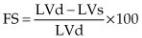
where LVd = left ventricular diastolic dimension and LVs = left ventricular systolic dimension.
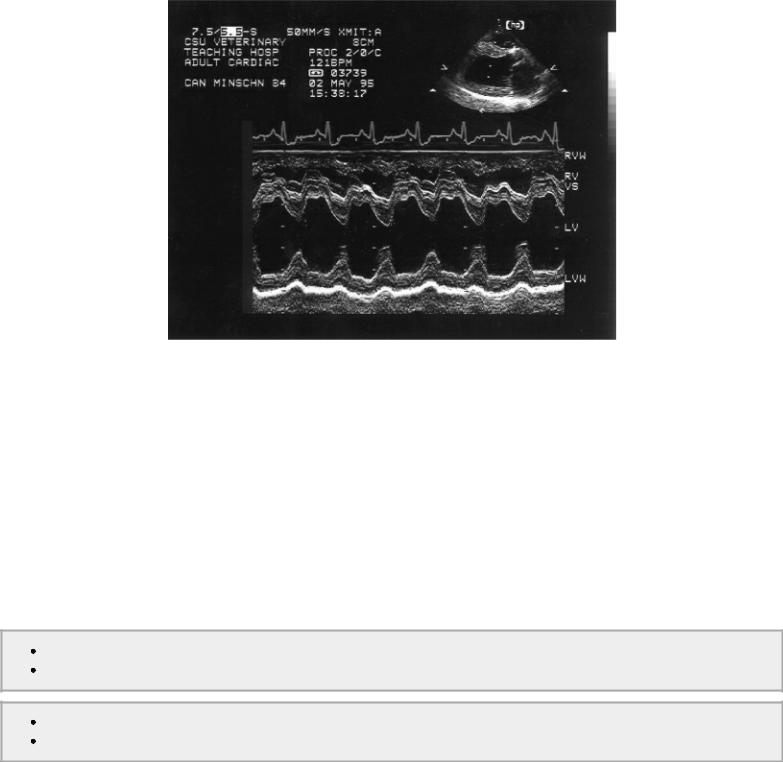
It is important to remember that fractional shortening is not a measure of contractility; it is a measure of function. The three primary factors that affect fractional shortening the most are preload, afterload, and contractility. Each one of these may individually or together affect FS (159). When fractional shortening is low it may be secondary to poor preload, increased afterload, or decreased contractility. Increased preload on the other hand tends to increase function as does decreased afterload (Figure 4.56) (157–159).
Fractional shortening is NOT only a measure of contractility.
Factors Affecting FS
Preload
Afterload
Contractility
Figure 4.56 Increased preload increases the fractional shortening in a heart that does not have myocardial dysfunction. RVW = right ventricular wall, RV = right ventricle, VS = ventricular septum, LV = left ventricle, LVW = left ventricular wall.
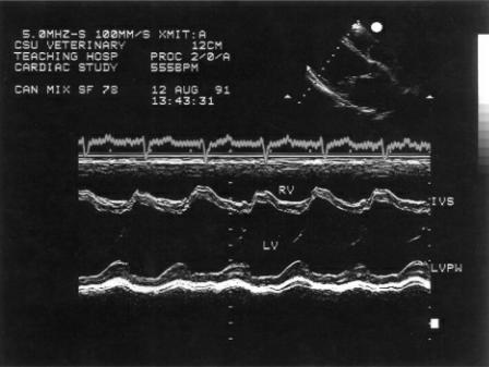
These factors may be hard to differentiate, but the M-mode measurements of size and Doppler flow analysis often aid in the determination. Increased left ventricular diastolic size stretches the myofibers and according to Frank Starling should increase the ability to shorten and increase fractional shortening. If fractional shortening is normal in the presence of increased preload, either increased afterload is inhibiting the ability to shorten or contractility is a problem (Figure 4.57). Decreased preload puts less stretch on the myofibers resulting in decreased ability to shorten and a poor fractional shortening. Hypertrophy that exceeds the normal chamber size to wall thickness ratio is consistent with chronically increased afterload (usually hypertension) or significantly decreased preload, which creates the appearance of hypertrophy (pseudo hypertrophy) simply due to a lack of distension (159). If hypertension is acute or acute on chronic there may be a decrease in fractional shortening, which is unrelated to contractility.
↑ preload = ↑ FS ↓ preload = ↓ FS
↑ afterload = ↓ FS ↓ afterload = ↑ FS
Figure 4.57 Fractional shortening in this heart is low normal and in the presence of the volume overload this suggests that the myocardium is failing. High afterload may also decrease fractional shortening. RV = right ventricle, IVS = interventricular septum, LV = left ventricle, LVPW = left ventricular wall.
Exercises involving measurements of size and function are found at the end of the chapter. The effects of preload, afterload, and contractility are evaluated in each of these cases. Fractional shortening is not correlated to body surface area or weight (15,17–19,21,42,44,46,47,49–67,69–73,75– 78).
Volume, Ejection Fraction, and Cardiac Output
Left Ventricle
Many equations for volume measurement exist. All are reliable measures of volume in the normal heart in man, and several have been shown to be valid in dogs and horses as well. The problem with most of these equations however is that they are not always applicable in the diseased heart. Twodimensional assessment of volume and output is more accurate, but it is also more time consuming. The ASE has listed recommendations for the determination of left ventricular volume and cardiac output in man (28). Two-dimensional echocardiography is recommended because of the limited view of the heart in M-mode views. The one dimension may not be representative of the left ventricular chamber as a whole. This is clearly a more important factor in man where ischemic heart disease may distort the chamber configuration dramatically. Many studies in man however have shown good comparisons between volume measured noninvasively and volume measured by applying the Teicholz equation to the normal LV M-mode image (163,164).
There are several studies that show a high correlation between M-mode derived volumes and cardiac output when using the Teicholz method in normal dogs (165,166). The Teicholz equation and its use to calculate ejection fraction (EF) and stroke volume (SV) (Equations 4.9, 4.10, 4.11, 4.12) is based upon the assumption that the left ventricular chamber is an ellipse and is as follows:
Equation 4.9 
Equation 4.10 
Equation 4.11 
Equation 4.12 
where LVd is left ventricular diastolic dimension and LVs is left ventricular systolic dimension. Correlation to invasive methods for deriving volume with this formula from the M-mode left ventricular image are high at .93 and .87 (165,166). Uehara found better correlation to true ejection fraction when using M-modes derived from transverse left ventricular two-dimensional images as opposed to long-axis views. This view is easier to obtain and the M-mode cursor is also easier to place correctly on this view. The inexperienced sonographer will undoubtedly find it easier and therefore often more accurate to obtain the M-mode images from transverse planes.
Left ventricular volume overload changes the geometry of the left ventricular chamber making it more spherical, and the M-mode derived left ventricular volume calculations are no longer accurate since the Teicholz equation does not take into account these geometric alterations (167). Calculation of systolic volume using the Teicholz equation results in a larger estimation of volume compared to methods that use two-dimensional images (167).
Similar results are not found in normal cats (168). Although correlations using the Teicholz equation are not terrible under resting conditions with the cat under anesthesia (r = .89), when varying drugs were used to enhance or diminish cardiac output, the correlation diminished considerably to .71 and .84, respectively. The small dimensions of the feline heart provide little room for error and probably play a role in these results.
Systolic and diastolic volume indices are used to unify ventricular size with respect to body size. Divide the systolic or diastolic volume by the animal’s body surface area to derive the index. The index can be used to compare the ventricular diastolic or systolic volume between dogs irrespective of size. An M-mode derived systolic volume index <30 ml/m2 and a diastolic volume index less than 100 ml/m2 are considered normal in all breeds and sizes of dog (167,169).
M-mode volume calculations in the horse show that the cube method, which uses the M-mode measured diameter of the left ventricular chamber, is quite accurate (r2 = .94) and easy to use in vitro studies (30). When ventricular length was derived from a ratio, as seen below, the correlation dropped slightly to .90. Values were just slightly less accurate than those that used two-dimensional images. Equations 4.13 and 4.14 show the calculations for this M-mode method:
Equation 4.13 
Equation 4.14 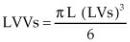
where L = ventricular length. Length may be obtained from the two-dimensional long-axis image and measured from apex to mitral annulus or length may be calculated as a ratio of diameter to length developed from in vitro studies and is derived as follows (Equations 4.15, 4.16):
Equation 4.15 
Equation 4.16 
where LVLd and LVLs = left ventricular length during diastole and systole, respectively. Ejection fractions and cardiac output are calculated as shown above.

Right Ventricle
The crescent-shaped right ventricular chamber is hard to see completely in echocardiographic imaging planes. Most evaluation of right ventricular function is qualitative in both man and animals (24). Estimates of volume and ejection fraction in the right ventricle are inaccurate. Right ventricular function has been assessed by calculating fractional area percent change (FAC) in man. This is obtained from apical four-chamber views and correlates well with MRI ejection fraction in people with normal and diseased hearts (24). Tricuspid annular motion and myocardial performance indices, imaging of the vena cava, and pulmonary artery pressure assessment using tricuspid regurgitant velocity are all more commonly used to assess right ventricular function (170,171). These indices and parameters are discussed later in this chapter.
Systolic Time Intervals
Systolic time intervals reflect systolic function (109,172). M-mode systolic time intervals (STI) include left ventricular ejection time (LVET), left ventricular pre-ejection period (PEP), velocity of circumferential shortening (VCF), and left ventricular ejection time to pre-ejection period ratio (LVET/PEP) (Figure 4.39, 4.42).
Systolic time intervals may be better indicators of left ventricular systolic function than fractional shortening and have been shown to be as accurate as invasive methodology in humans for the assessment of left ventricular performance (109,173,174). Just as with fractional shortening however, the STI are not indicators of contractility but rather function. They are affected by preload, afterload, and contractility. In general, decreased preload without any concurrent pathology will increase PEP, decrease LVET, and increase PEP/LVET (109,110,174). Increases in preload tend to shorten PEP, increase LVET, and decrease PEP/LVET (109,110,173,174). Afterload reduction will decrease PEP, increase LVET, decrease PEP/LVET, and increase VCF (109,110,173,174). Increases in afterload tend to increase PEP, increase LVET, and decrease VCF (109,110,173,174). Table 4.1 summarizes how preload and afterload affect the systolic time intervals.
Systolic Time Intervals
PEP and LVET in the normal heart
Preload dependent
Increased preload
Decreases PEP
Increases LVET
Decreased preload
Increases PEP
Decreases LVET
Afterload Dependent
Increased afterload
Increases PEP
Increases LVET
Decreased afterload
Decreases PEP
Increases LVET
Table 4.1 Effects of Preload and Afterload and Heart Rate on Systolic Time Intervals

PEP = pre-ejection period, LVET = left ventricular ejection
time, Vcf = velocity of circumferential shortening, ↑ = increase or lengthen, ↓ = decrease or shorten
Data from Atkins CE, Snyder PS: Systolic time intervals and their derivatives for evaluation of cardiac function. J Vet Int Med 6:55, 1992.
When afterload is increased, the heart’s workload is increased, and as a result, the time it takes to generate enough pressure within the left ventricle before the aortic valve can open is longer. This time corresponds to the pre-ejection period. The rate at which the heart can contract in the face of high afterload is also reduced, which results in reduced VCF. Decreases in afterload however allow the left ventricle to function with greater ease, and the force necessary to open the aortic valve is reached sooner resulting in decreased PEP. The rate at which the heart can contract is also faster when the workload is reduced and VCF is increased.
Changes in preload can be approached the same way. High preload or volume within the left ventricle allows the Frank Starling mechanism to come into play as fibers are elongated and function is enhanced. This shortens PEP and increases LVET. Decreased preload however does not allow enough force to be generated by fibers that are not at optimum length, and PEP is increased. By the same token, volume within the left ventricle affects LVET and a reduction in volume and force of contraction will decrease LVET. Table 4.1 summarizes this information.
There are many applications for systolic time intervals within the diseased heart, and these are listed in Table 4.2. There are limitation to their use however since heart rate and loading conditions do affect them significantly (109). Contractility cannot be evaluated accurately without first analyzing the effects of preload and afterload on the heart.
Table 4.2 Systolic Time Intervals in Various Cardiac Diseases
PEP = pre-ejection period, LVET = left ventricular ejection
time, Vcf = velocity of circumferential shortening, ↑ = increase or lengthen, ↓ = decrease or shorten
Data from Atkins CE, Snyder PS: Systolic time intervals and their derivatives for evaluation of cardiac function. J Vet Int Med 6:55, 1992.
Mitral and Tricuspid Annular Motion
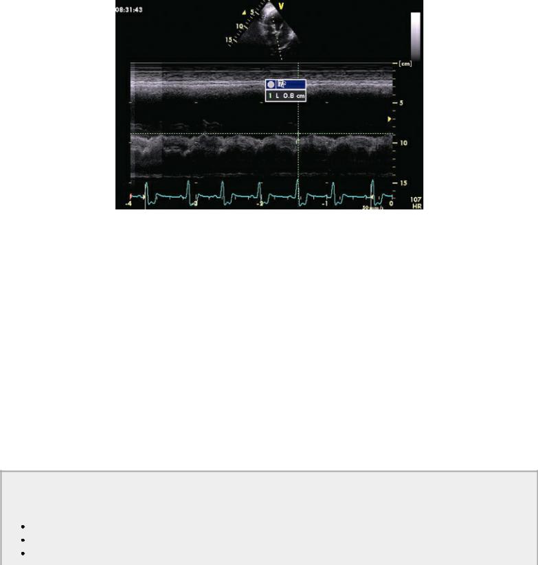
Mitral annular motion (MAM) is correlated with ejection fraction (175,176). Obtained from apical four-chamber views using M-mode of the septal side of the mitral annulus, this measurement shows a strong nonlinear correlation with ejection fraction in healthy people and dogs and in individuals and dogs with heart disease (Figure 4.58) (175,176). Mitral annular motion decreases with age but does so only in patients with normal ejection fractions, while age does not affect MAM in the patient with depressed ejection fraction (175,176).
Figure 4.58 Mitral annular motion (MAM) is correlated with ejection fraction. Here decreased MAM (.8 cm) is seen in this dog with dilated cardiomyopathy.
Mitral annular motion in normal dogs ranges from .46–1.74 cm. There is a strong relationship with body weight. Dogs weighing less than 15 kg have a 95% confidence interval for MAM of .65–.75 cm with all dogs in this group having MAM above .45 cm. The 95% confidence intervals for dogs ranging from 15–40 kg and for those greater than 40 kg are 1.03–1.13 cm (all above .80 cm), and 1.21–1.81 cm (all above 1.2 cm), respectively. This parameter may be more useful indexed to body weight because of this strong linear relationship between body size and annular motion (r = .800, p = <.001). The regression equation for the relationship between MAM and body weight is as follows (Equation 4.17):
Equation 4.17 
where BW = body weight in kg (176).
Trying to overcome the strong relationship to body weight, MAM can also be indexed to body weight by dividing MAM by body surface area. These values range from 1.47–1.83 cm/m2, 1.04–1.18 cm/m2, and .89–1.17 cm/m2, in dogs less than 15 kg, dogs ranging from 15–40 kg and dogs over 40 kg, respectively. Dogs less than 15 kg have statistically higher indexed MAM than larger dogs, but the index does not show any advantage over using absolute MAM values (176).
MAM decreases with decreased ejection fraction.
Normal MAM
1.47–1.83 cm/m2 (<15 kg dogs) 1.04–1.18 cm/m2 (15–40 kg dogs)
.89–1.17 cm/m2 (>40 kg dogs)

Calculating a MAM percent by using fractional shortening of the long and short axis is another effort to normalize this index (Equation 4.18). MAM percent has an insignificant relationship with body weight and is between 40 and 45% in all dogs. The equation is as follows:
Equation 4.18 
where LVd is the left ventricular diastolic dimension from the M-mode and LVs is the systolic M- mode dimension.
Tricuspid annular motion or tricuspid annular plane systolic excursion (TAPSE) using M-mode on apical four-chamber imaging planes has been evaluated in man. The normal range in man is 1.5–2.0 cm. An excursion of less than 1.5 cm is associated with a poorer prognosis in human patients in leftsided congestive heart failure secondary to dilated cardiomyopathy and in patients with pulmonary hypertension (177,178).
Two-Dimensional Measurement of Systolic Function
Volume, Ejection Fraction, and Cardiac Output
Volume determination using two-dimensional echocardiography is a labor intensive process and requires precise identification of left ventricular planes and evaluation through at least five cardiac cycles. It is not a calculation that is routinely done during a clinical exam. It is however used in research and will briefly be described here. Formulas are used that determine the ventricular volume at end diastole and end systole. A percent change is then calculated that equals the ejection fraction.
While M-mode methods of volume determination in the cat, dog, and man with heart disease have poor correlation with more invasive methods of volume determination and is not thought to be clinically useful in the setting of heart disease, volume determination using two-dimensional echocardiographic images is shown to be accurate in normal and abnormal human hearts (28,32,167,168,179). Factors that affect the accuracy of two-dimensional volume calculations include endocardial dropout, the type of cardiac disease present, the use of a foreshortened ventricular chamber, mathematical assumptions, and the use of more advanced technology such as tissue harmonic imaging (24,180). These two-dimensional equations are based upon the fact that the normal left ventricle is elliptical. The most commonly used formula for volume determination in man and that which is recommended by the ASE is the modified Simpson’s rule (28). This formula shows the best correlation with actual left ventricular volumes in the diseased heart appearing to be relatively unaffected by changes in ventricular geometry. Even if volume is not accurate in some diseased hearts, the calculation may be used in an individual to follow progression or regression of left ventricular volume. It should also be noted that ejection fraction does not imply forward stroke volume. Ejection fraction is a measure of volume leaving the left ventricle regardless of whether it flows through the aorta, a shunt, or the mitral valve. End diastolic and end systolic planes are used for volume calculations. End diastolic frames are defined as the frame just before the mitral valve closes or the first frame into the QRS complex. End systolic frames are identified as the frame just before the mitral valve opens or the smallest chamber size (24).
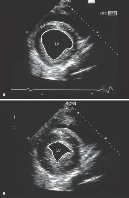
The modified Simpson’s rule involves tracing the left ventricular endocardial border, and computerized calculations treat the ventricle as a stack of discs (Figure 4.59). A volume for each disc is calculated and summated for the total left ventricular volume. Other terms for this method of
volume measurement are the method of discs or the disc summation method. Ideally two long-axis apical planes should be used, the apical four-chamber and the apical two-chamber planes. Two imaging planes will more accurately account for any irregularities of the left ventricular chamber. The planes should maximize length and width. A true apex is difficult to obtain in both man and animals, and in actuality usually the lateral wall of the ventricle is really seen as opposed to the apex. An optimal left ventricular length is usually about two times its width. When ventricular size is maximized, the small amount of volume not accounted for is minimal and negligible. After tracing along the endocardial surface of the left ventricular chamber in both planes, following the mitral annulus at the heart base, computation packages in the ultrasound equipment will divide the ventricle into discs and perform the volume calculation shown in (Figure 4.59).
Figure 4.59 (A) Biplane volume calculations are performed on apical twoand four-chamber views. The endocardial surface of each view is traced, and volume is calculated by summating the areas of 20 or more discs. Internal software divides the length of the chamber (L) into the discs and applies the equation shown. (B) Single plane volume calculation involves tracing the area of a single apical left ventricular plane as well as measuring its length (L) and applying the equation as shown. Adapted from Schiller N.B., Shah P.M., Crawford M., et al.: Recommendations for quantitation of the left ventricle by two-dimensional echocardiography: American Society of Echocardiography Committee on Standards Subcommittee. J Am Soc Ech 2:358–367, 1989.

When two views are not possible, a single apical plane may be used (Figure 4.59). The use of one plane in veterinary medicine is potentially more accurate than in man where regional wall motion abnormalities secondary to coronary artery disease are common and affect volume calculations. An area length computation is used to calculate volume when one apical image is used. The area of the left ventricle is determined by tracing the endocardial surface, and the length is measured from the mitral annulus to the apex. The equation is as follows (Equation 4.19):
Equation 4.19 
and is shown in Figure 4.59, where A = area of the LV chamber, and L = ventricular length, both measured on the apical four-chamber image.
A study in dogs using the bullet formula for volume determination found good correlation between echocardiographically determined ejection fractions in anesthetized dogs and gated equilibrium radionuclide ventriculography (166). This formula has also been used in dogs where echocardiographically determined volumes were compared to postmortem values (181). The
correlation to invasive measures of volume is high at .97. The bullet method is so called because it assumes a bullet-shaped left ventricular chamber with a wider base and rounded apex. The bullet method utilizes transverse left ventricular dimensions and left ventricular length. Transverse images at the level of the chordae are traced in diastole and systole in order to calculate areas (A) (Figure 4.60). Left ventricular length (L) is measured on the right parasternal long axis from the apex of the ventricular to the mitral aorta junction (Figure 4.20). The bullet formula (Equation 4.20) is:
Equation 4.20 
where LVV is left ventricular volume.
Figure 4.60 Volume determination based upon the Bullet formula involves tracing the endocardial surface of the left ventricle on right parasternal transverse planes at the level of the chordae tendinae during (A) diastole and (B) systole. LV = left ventricle.
Transverse measurements of the horse’s heart have been used to determine left ventricular volumes with good correlation to invasive methods of volume calculation. These results were obtained in vitro, and their accuracy in the living horse still needs to be determined (30,182).
An ellipsoid model of volume determination in the horse proves to be the simplest with no loss in accuracy (30). This involves tracing endocardial and epicardial boundaries of the left ventricular transverse plane at the level of the papillary muscles (Figure 4.61). Volumes are calculated for systole and diastole. Equation 4.21 is applied:
Equation 4.21 
where A = area, L = length. Left ventricular length cannot be determined with any accuracy in the equine heart. An average ratio of length to diameter was determined, and this value of 1.46 is applied to the diameter in order to determine length.
Figure 4.61 Volume in the equine heart involves tracing the left ventricular endocardial surface on right parasternal transverse planes at the level of the papillary muscles as opposed to the chordae during (A) diastole and (B) systole. LV = left ventricle.
Systolic and diastolic volume index calculation using both area length and Simpson’s rule methods yield similar results and take into account the changing geometry encountered with volume overload. A systolic or diastolic volume index is derived by dividing the volume calculated by either of these methods by the dog’s body surface area. A systolic volume index of less than 30 ml/m 2 and a diastolic volume index less than 70 ml/m2 are considered normal in the dog (167).
Spectral Doppler Evaluation of Systolic Function
Volumetric Flow
Conservation of mass is a physical principle used in Doppler to calculate volumetric flow. This principle states that mass in equals mass out. Since mass is equal to density (D) × volume (V) × area (A), and density is constant, the equation can be modified to (Equation 4.22):
Equation 4.22 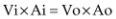
where Vi = volume in , Vo = volume out, Ai = area in, and Ao = area out. The continuity equation (Equation 4.23) is derived from this principle.
Equation 4.23 
where Q = flow. In other words, flow into the heart equals flow out of the heart.
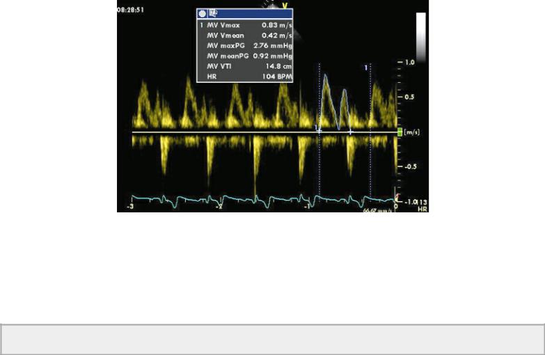
Volume of flow is calculated by tracing the flow profile and determining the flow velocity integral (FVI) (area under the curve, also called time velocity integral [TVI], and velocity time integral [VTI]) (Figure 4.41). FVI is multiplied by the area of the vessel, valve, or orifice through which flow volume is being calculated. The result is stroke volume through that path in the heart. This measurement can be done at any of the four valves (183–187). Flow velocity integrals at the mitral valve should use profiles that maximize peak E and A velocities (Figure 4.62).
Figure 4.62 The velocity time integral (VTI) is measured by tracing the mitral inflow profile, which maximizes both the E and A peaks. Here the peak E velocity (MV Vmax) is .83 m/sec and the MV VTI is 14.8 cm.
The FVI is directly proportional to stroke volume, and its value is calculated by the machine once the flow profile is traced. It can be measured manually by applying Equation 4.24:
Equation 4.24 
where V = peak velocity and ET = ejection time.
VTI is directly proportional to stroke volume.
The other part of the continuity equation states that the area of the vessel or orifice must be calculated. Measurement of volumetric flow assumes that the blood is flowing thorough a circular orifice since area calculations are based on a circle. Cross sectional area (CSA) is calculated by using Equation 4.25:
Equation 4.25 
where r = radius and Π = 3.14. The radius is obtained by measuring the diameter of the vessel or
annulus involved in the flow calculation. Studies have tried to determine which location is the best for measuring valve areas and still this is the greatest source of error in this method of calculating stoke volume and cardiac output. Although aortic flow has been studied and validated in dogs, pulmonary, mitral, and tricuspid flows need more evaluation.
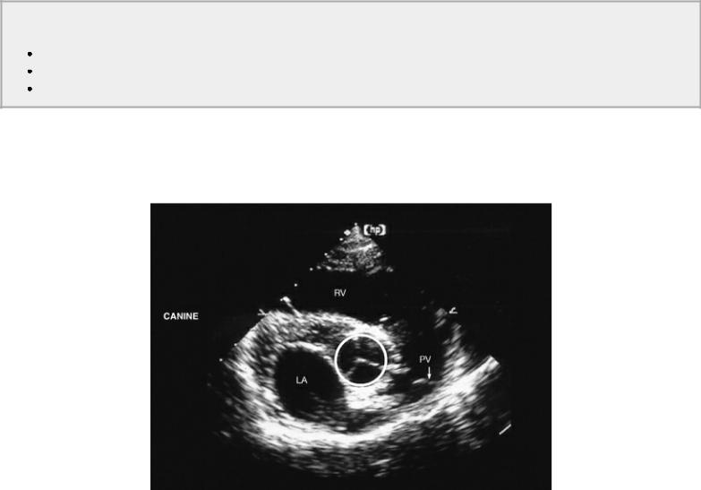
Studies in dogs have measured cardiac output by measuring area of the aorta from several imaging planes using both trace and diameter methods (100,165). Calculations based upon the same FVI and areas calculated from the three views for aorta showed that the highest correlation (r = .93) when compared to thermodilution-derived cardiac output was when aortic area was measured by tracing the lumen of the aorta on a right parasternal transverse plane of the heart base (Figure 4.63) (165). This makes Doppler-derived left ventricular stroke volume calculations a fairly valid assessment of left ventricular function.
Cross-sectional Areas
Trace right parasternal aortic root cross sections
Use apical four-chamber for mitral annulus
Use diameter of PA on transverse planes
Figure 4.63 Although there are many places to measure the aorta, tracing the aortic lumen on right parasternal transverse views of the heart base shows the highest level of accuracy in assessing volumetric flow. RV = right ventricle, LA = left atrium, PV = pulmonic valve.
Measurement of output from the right side is variable and has poor correlation (r = .31) with invasive measures of output (100,165). This is primarily due to variability in diameter measurements of the pulmonary artery because of poor resolution of the lateral walls (Figure 4.64). Studies in man show higher correlations with invasive measures of output, but they still are generally less accurate than flow measured at the aorta (188,189). Averaging several beats is important in order to account for the variation in flow caused by respiration.
Figure 4.64 Pulmonary artery diameter is measured on right or left parasternal images of the pulmonary artery at the level of the pulmonic valve. RV = right ventricle, RA = right atrium, LA = left

atrium, PA = pulmonary artery, RMPA = right main pulmonary artery.
There is great variability in stroke volume calculation at the mitral valve because of error introduced while measuring the mitral annular area. Two methods are used in man, and they have been studied in dogs (185,190). The annulus can be measured by either tracing the orifice from transverse views or by measuring the diameter of the annulus.
Tracing the area of the orifice the largest mitral valve area is used on transverse views of the left ventricle (Figure 4.65). Unfortunately mitral flow is biphasic, and a mean flow area as opposed to maximal flow area should be calculated. This is done by tracing the transmitral flow profile and determining a ratio of mean to maximal leaflet separation. The two-dimensional area is multiplied by ratio area in order to obtain the mean mitral area for diastole. This was studied in open chested dog and found to have a high correlation or r = .97 to true area (189). It is difficult to apply however, and varying results are seen.
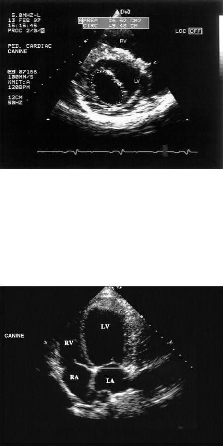
Figure 4.65 Mitral valve area may be measured from transverse images by tracing the largest area. Here the area measurement is 6.52 cm2. RV = right ventricle, LV = left ventricle.
The mitral annulus can be measured from apical four-chamber views (Figure 4.66). To account for changes in annular size during diastole, several frames need to be measured and averaged after the valve opens. Both circular equations (Equation 4.25) and elliptical equations (Equation 4.26), when two planes for diameter (d) are interrogated, have been applied to area calculations (185,191).
Equation 4.26 
Figure 4.66 Mitral valve annular size can be measured on left parasternal apical four-chamber views. LV = left ventricle, RV = right ventricle, RA = right atrium, LA = left atrium.
Both show good correlations (r = .99 in circular method) with actual area. At this time the diameter measurement using the circular equation appears to be the easiest and no less accurate than any other method. Flow measurement at the tricuspid valve is not well studied, and results are variable enough that it is not routinely used in people or reported in animals. Stroke volume (SV) is finally calculated by multiplying the FVI by the area of the vessel or annulus (Equation 4.27).
Equation 4.27 
Errors in measuring diameter are squared when inserted into area calculations. Using the FVI itself is a valid assessment of increased or decreased flow in situations where diameter measurements are questionable. Increases in FVI may suggest increased volume, as in a shunt, while decreases in FVI can represent poor flow. Exercises at the end of the chapter involve the application of flow velocity integrals.
Systolic Time Intervals
Research in animals has shown that the rate of acceleration during ventricular ejection is an indicator of systolic function (Figure 4.43). The force created within the left ventricle in order to open the aortic valve affects the rate at which maximum velocity is reached. This variable has been studied in dogs, and in man, it is thought to be one of the better indicators of systolic function (192–194). It has been used to chart changes in left ventricular function. It is dependent upon heart rate and systolic load however. Mean aortic flow acceleration is 32 cm/sec2 in dogs (95).
Ejection time or flow time and pre-ejection period may both be measured from aortic or pulmonary flow profiles, and this method has been described earlier (Figure 4.42). Their application is the same as when the values are derived from M-mode images.
Myocardial Performance Index
The myocardial performance index (MPI) is an index of global myocardial function and includes both diastolic and systolic time intervals. The MPI is also called the Tei index. In man, this index can provide prognostic information in patients with valvular aortic stenosis, dilated cardiomyopathy and mitral regurgitation (195,196). The Tei index correlates well with both systolic and diastolic function of the right and left ventricle in dogs and can be used to assess overall global function (196,197). The MPI can identify subclinical dilated cardiomyopathy in the Newfoundland dog and identifies dysfunction in dogs with tricuspid regurgitation, mitral regurgitation and pulmonary hypertension (197–199).
This measurement uses ventricular ejection time and the isovolumic periods (contraction and relaxation) to derive an overall assessment of global ventricular function. Isovolumic relaxation time and isovolumic contraction time are added together and divided by the ejection time (Figure 4.67). Using pulsed-wave Doppler, the time intervals are derived from different cardiac cycles. The time from closure of the AV valve to opening is the sum of the systolic time period and the two isovolumic time periods (Figure 4.68). Ejection time is obtained from trans aortic or pulmonary flow from beginning of flow to the end of flow using the spectral trace (Figure 4.68). Subtracting the ejection time from the closure to opening time of the AV valve provides the sum of the isovolumic relaxation and contraction time periods. Equations 4.28 and 4.29 are used to calculate the myocardial performance index as follows:
Equation 4.28 
Equation 4.29 
where LV is left ventricle, RV is right ventricle, IVRT is isovolumic relaxation time, IVCT is isovolumic contraction time, MCO is mitral valve closing to opening time, TCO is tricuspid valve

closure to opening time, and LVET and RVET are left and right ventricular ejection times, respectively.
MPI (Tei Index)
Assesses global ventricular function
Using PW Doppler or TDI
Color TDI-derived MPI higher than PW-derived MPI
Figure 4.67 The Tei index (also called myocardial performance index [MPI]) uses ventricular ejection time and the isovolumic periods (contraction and relaxation) to derive an overall assessment of global ventricular function. Isovolumic relaxation (IR) time and isovolumic contraction (IC) time are added together and divided by the ejection time (LVET). Often mitral closure to opening (MCO) is measured and ejection time is subtracted from this time period in order to derive the sum of the isovolumic time intervals. MV = mitral valve, AO = aorta.
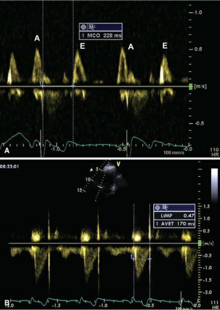
Figure 4.68 (A) Mitral closure to opening (MCO) measured on a pulsed-wave transmitral flow. (B) Aortic ejection time (AVET) measured from a pulsed-wave aortic flow profile. LMIP = left index of myocardial performance.
Myocardial performance index can also be calculated from tissue Doppler evaluation of the longitudinal free wall or septum on apical four-chamber views of the heart. The advantage to deriving the MPI using TDI is that the same cardiac cycle can be used since TDI records myocardial motion during systole and diastole wherever the pulsed-wave gate is placed. Figure 4.69 shows how MPI is derived from tissue Doppler images. Tissue Doppler MPI may help overcome errors in evaluation secondary to variations in heart rate when PW is used at different points in time. Color-tissue Doppler-derived LV MPI is slightly higher than PW TDI even though they have similar values with a significant correlation between them (.70 r value) (200).
Figure 4.69 (A) Using pulsed-wave tissue Doppler images, the time periods for calculation of myocardial performance index are shown. (B) Time periods used for calculation of myocardial performance index are shown on this color-tissue Doppler image. IVR and IRT = isovolumic relaxation time, IVC and ICT = isovolumic contraction time, LVET = left ventricular ejection time, S′ = systolic myocardial motion, E′ = early diastolic myocardial motion, A′ = late diastolic myocardial motion.
The Tei index correlates well with systolic and diastolic function of the right and left ventricle in dogs and cats (197,199,201). Studies in anesthetized dogs and cats have shown that increases in systolic function after inotropic infusion can be detected by decreased myocardial performance index derived from PW Doppler and TDI at both the free wall and at the septum. Septal TDI-derived MPI had better correlation with LV systolic function than free wall TDI derived MPI (197,202).
Both TDIand PW-derived MPI correlate significantly with left ventricular filling pressure and may be useful in the assessment of global cardiac function in dogs with left ventricular failure. Decreases in preload decrease ejection times but increase the isovolumic time periods, resulting in increased MPI. Acute increases in preload that increase ejection time will decrease MPI. Tissue Doppler-derived MPI appears to be more accurate than PW-derived Tei index in assessing changes in function caused by changes in preload (199,202).
Most studies have shown pulsed-wave derived left ventricular MPI to be independent of heart rate, blood pressure, body weight, body surface area, sex, and age in dogs and cats (198,199,202,203). One study showed the PW-derived left ventricular MPI to increase with advancing age in dogs. This is thought to be secondary to age-related increases in ventricular relaxation time (196,199). Right

ventricular Tei index is also unaffected by age, heart rate, and body weight (197,204).
The Tei index appears to be preload and BP independent but is significantly affected by acute changes in loading conditions (205). In dogs with mitral regurgitation secondary to degenerative valve disease, the Tei index remained normal unless systolic dysfunction was present (199). Volume overloading of the right ventricular chamber does not affect tissue Doppler-derived MPI in dogs, and the presence of tricuspid regurgitation does not affect the MPI in children (140,206). It is a sensitive indicator of acute increases in afterload, however, which causes the Tei index to increase. Increased values for both right and left ventricular MPI are indicative of myocardial dysfunction when changes in load are chronic.
Increased MPI = poor function
Independent of
HR
BP
Weight
Age
Sensitive to acute changes in afterload
Preload independent
Tissue Doppler Evaluation of Systolic Function
Left Ventricle
Tissue Doppler provides information regarding myocardial velocity in very specific selected areas of the myocardium. A pulsed-wave gate placed over the myocardium shows both systolic (Sm) and diastolic myocardial motion (Em and Am), which is used to evaluate function (Figure 4.70) (126). When color-tissue Doppler imaging is used, systolic and diastolic gradients along the septum and lateral wall on apical views and between the epicardium and endocardium on transverse views can be evaluated.
Figure 4.70 Tissue Doppler time intervals associated with myocardial function include the following: Q-S′ (the time interval from the beginning of the QRS complex to the beginning of S′), Q-peak S (the time interval from the beginning of the QRS complex to peak velocity of S′), Q-end S′ (the time interval from the beginning of the QRS complex to the end of S′), and duration (dur) of S′, IVC = isovolumic contraction period, IVR = isovolumic relaxation period, S′ = systolic myocardial motion, E′ = early diastolic myocardial motion, A′ = late diastolic myocardial motion.

Tissue Doppler time intervals associated with systolic myocardial function include Q–Sm (the time interval from the beginning of the QRS complex to the beginning of Sm), Q–peak Sm (the time interval from the beginning of the QRS complex to peak velocity of Sm), Q–end Sm (the time interval from the beginning of the QRS complex to the end of Sm), and duration of Sm (Figure 4.70). These are measured on both sides of the mitral annulus on the apical four-chamber-imaging plane. There are significant inverse relationships between Q–Sm and ejection fraction and between Q–end Sm and ejection fraction, and a significant positive relationship between ejection fraction and duration of Sm. These TDI indices are heart rate affected, and all of these time intervals should be corrected for heart rate by dividing the parameter by the square root of the R-to-R interval.
Systolic failure in dogs and man with dilated cardiomyopathy results in a decreased systolic gradient using color TDI between the subendocardium and subepicardium on transverse images and a decreased gradient between basal and apical free-wall systolic motion on apical four-chamber planes (207,208). Color TDI in a Great Dane with subclinical myopathy revealed a depressed radial epicardial to endocardial Sm gradient. This was detected before any definitive two-dimensional, M- mode or clinical signs of dilated cardiomyopathy were present (209). A Golden Retriever with subclinical DCM associated with muscular dystrophy showed decreased color TDI Sm gradients along both longitudinal and radial myocardial segments (210).
Pulsed-wave TDI shows decreased longitudinal Sm at the base of the left ventricular wall in both subclinical and overt dilated cardiomyopathy in Doberman Pinchers (211). Peak systolic annular motion of the myocardium along the longitudinal axis at both the free wall and septal mitral annulus decreases with even mildly depressed systolic function in dogs (212). In man, depressed Sm annular velocity is a sensitive indicator of depressed systolic function despite echocardiographically derived normal ejection fractions (213). Mitral annular systolic velocity correlates well with left ventricular systolic function even in human patients with severe mitral regurgitation and can be used as a predictor of postoperative development of reduced ejection fraction (214). This means that Sm can detect subclinical systolic dysfunction in patients with mitral regurgitation (214). Studies in dogs show that increases in systolic function after inotropic infusion can be detected by increases in annular Sm and decreases in myocardial performance index derived from PW TDI at both the free wall and at the septum. Septal Sm had better regression correlation with systolic function than the free wall Sm (215). Experimental studies have shown that decreases in systolic function after pacing induced heart

failure correlates well with systolic annular motion (Sm) (212). In dogs, subclinical dilated cardiomyopathy can be diagnosed by decreases in Sm (208,210,216).
Systolic failure has also been documented in cats with hypertrophic cardiomyopathy. Depressed color TDI Sm all along the left ventricular lateral wall and septum on apical four-chamber views has been documented. There is also decreased acceleration of systolic myocardial motion in these cats. This is seen in cats with HCM despite normal to elevated fractional shortening (217).
Color TDI documented postsystolic contraction may be seen with systolic failure. This late systolic motion occurs after the T wave during the isovolumic relaxation time period. This late delayed contraction velocity is usually greater than twice the normal systolic velocity. As a result, Em is not present (217,218). The underlying cause of this postsystolic contraction is poorly understood, but it is indicative of systolic dysfunction (217,218).
Tissue Doppler Imaging
Decreased Systolic Function
Decreases Sm
Decreases radial gradient
Decreases longitudinal gradient
Postsystolic contraction may be present.
Right Ventricle
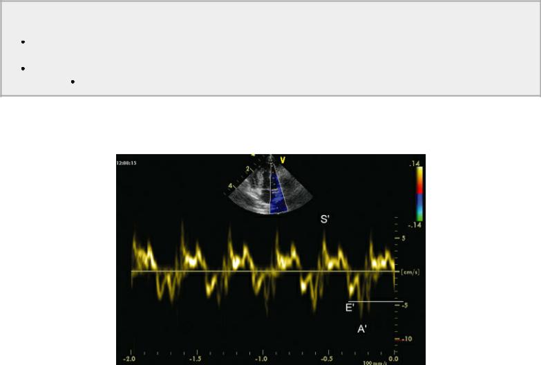
Tissue Doppler examination of systolic annular motion is also used in the right ventricle. Decreased PW TDI systolic annular velocity correlates well with decreased right ventricular ejection fraction in man (219). Assessment of longitudinal systolic function using two-dimensional color TDI of the right ventricle involves placing a pulsed-wave gate at the lateral tricuspid valve annulus on a modified left parasternal apical four-chamber view of the heart (Figure 3.67). Parameters that reflect systolic function include peak systolic annular motion (Sm), isovolumic contraction time (ICT), ejection time (RVET), and the myocardial performance index (MPI or Tei). Reduced systolic annular velocity is associated with right ventricular systolic failure, myocardial infarction, and pulmonary hypertension in man (220). Systolic annular motion of the right ventricular wall correlates well with RV function regardless of the presence or absence of pulmonary hypertension in man (221). In the dog, color TDI imaging of the right ventricular wall has been shown to be useful in diagnosing the presence of pulmonary hypertension when a pressure gradient cannot be obtained from tricuspid regurgitant flow (222). Global TDI (Sm × Em:Am), Sm, and Em:Am are all significantly reduced in dogs with pulmonary hypertension.
Evaluation of Diastolic Function
Normal diastolic function allows the heart to fill appropriately at normal filling pressure. Diastolic failure is the result of increased resistance to filling and increased left ventricular filling pressure (156,223). Diastolic heart failure is the presence of congestive heart failure or symptoms in the face of normal systolic function. Diastolic dysfunction simply refers to the presence of myocardial alterations from normal during diastole but does not indicate anything regarding the patient’s clinical status (112). Research in man has shown that diastolic dysfunction often plays a large role in the clinical manifestation of heart failure. Systolic function may actually be normal in many patients with
congestive heart failure (224,225). Diastolic function of the heart is very complex and involves several interactive components. These include myocardial relaxation, atrial contraction, rapid and slow filling phases, loading conditions, the pericardial sac, and elastic properties of the heart. An explanation of all these factors is beyond the scope of this text, but there are excellent reviews devoted to the subject (111,114,117,118,154,226,227). The echocardiographic assessment of diastolic function as it applies to the clinical situation will be presented here and will incorporate the evaluation of isovolumic relaxation, transmitral valve flow, pulmonary venous flow, and tissue Doppler imaging. Assessment of diastolic function in specific cardiac diseases is covered in more detail in those chapters of this text.
Parameters of Diastolic Function
Isovolumic relaxation time
Pulmonary vein flow
Transmitral valve flow
TDI—Em, Am
Diastole extends from closure of the semilunar valves to closure of the atrioventricular valves. This roughly corresponds to the time period from the T wave on an electrocardiogram to the beginning of the QRS complex. Left ventricular relaxation is an active process requiring energy expenditure. After peak systole, left ventricular pressure drops, and once it drops below aortic pressure, the semilunar valve closes. At this point, a period of isovolumic relaxation begins. All valves are closed as left ventricular pressure continues to decline. The time that elapses from the end of ventricular ejection to when the mitral valve opens and diastolic flow into the left ventricle begins is the isovolumic relaxation period (Figure 4.71). No change in volume occurs and all valves are closed, but pressure decreases and the myocardium relaxes (112). Relaxation continues even after the mitral valve opens.
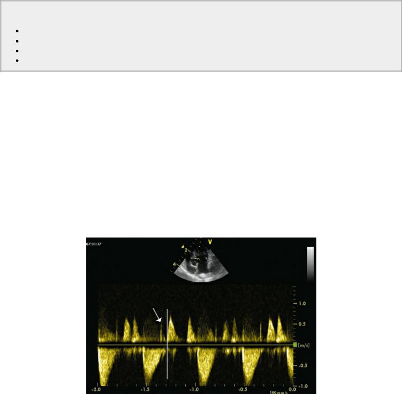
Figure 4.71 The time that elapses from the end of ventricular ejection (arrow) to when the mitral valve opens (vertical line) and diastolic flow into the left ventricle begins is the isovolumic relaxation period.
Filling of the left ventricular chamber has several phases: a rapid ventricular filling phase, a slow

ventricular filling phase, and filling secondary to atrial contraction. The peak flow velocity between the left atrium and left ventricle is determined by the pressure gradient between the two chambers. The Bernoulli equation cannot be directly applied to flow across the mitral annulus because of various factors including viscous forces, internal forces, and flow acceleration, but the pressure differentials during the various phases of diastole are reflected in the left ventricular inflow profile.
At the beginning of diastole, left ventricular pressure is lower than left atrial pressure, and there is a rapid inflow of blood into the left ventricle (Figure 4.72). This creates an increase in left ventricular pressure, and as left ventricular pressure equilibrates or even slightly exceeds left atrial pressure, flow velocity decelerates. During mid-diastole, blood passively flows into the left ventricle at a very low velocity. There is no measurable change in pressure during this phase of diastole. During the atrial contraction at the end of diastole, flow velocity accelerates but not to the degree of the rapid ventricular filling phase of early diastole. Most of left ventricular filling is completed by the end of the rapid ventricular filling phase (end of the mitral valve E peak) in the normal heart (114). Thus, peak E wave of the mitral valve reflects the pressure gradient between the left atrium and left ventricle at the beginning of diastole (112). As pressures equilibrate between the two chambers, a period of diastasis occurs and the time for pressures to equilibrate is reflected by the deceleration time of the E wave. Valve motion with atrial systole (A wave) reflects the pressure gradient between the left atrium and left ventricle at the end of diastole (112,121).
Figure 4.72 Transmitral valve flow is measured here. MV E Vel = mitral valve peak E velocity, MV DecT = mitral valve deceleration time, MV dec Slope = mitral valve deceleration slope, MV A Vel = mitral valve A velocity, MV PHT = mitral valve pressure half time.
Diastolic filling abnormalities may be secondary to impaired or delayed relaxation or decreased compliance within the left ventricle. When relaxation is impaired, left ventricular pressure remains high early in diastole, and left ventricular filling is delayed until later in the diastolic time period resulting in a greater contribution to left ventricular filling from the atrial contraction. Compliance of the heart is a reflection of its distensibility. A compliant ventricular chamber allows proper filling at normal pressure while a noncompliant ventricular chamber is stiff, and pressure elevates rapidly as the chamber fills. Compliance plays a larger role in late diastole when the ventricular chamber is already partially filled (117,118). Hypertrophy and ischemia are primary factors affecting relaxation,
while fibrosis, infiltrative processes, hypertrophy, and other structural abnormalities are the primary factors affecting compliance of the heart (112,114).
Impairment of diastolic function can produce backward or forward heart failure. Forward failure results from decreased ventricular volume secondary to restricted filling. Backward failure is the result of high left ventricular filling pressure reflected back into the left atrium. Other factors affecting ventricular filling include heart rate and rhythm and left atrial function. Rapid heart rates limit adequate left ventricular filling since early rapid filling and late diastolic filling phases coincide. Poor atrial function also diminishes late diastolic filling (112,117,118,228).
Impaired Relaxation
Abnormal myocardial relaxation results in decreased peak velocities in early diastole (E peak), increased A velocities, a low E:A ratio, increased deceleration times, and increased isovolumic relaxation times (Figures 4.73, 4.74) (112,117,118,186,223,228,229).
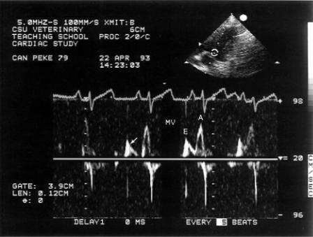
Figure 4.73 Abnormal myocardial relaxation in this dog results in decreased peak E velocity, increased A velocity, and longer deceleration time (arrow). MV = mitral valve.
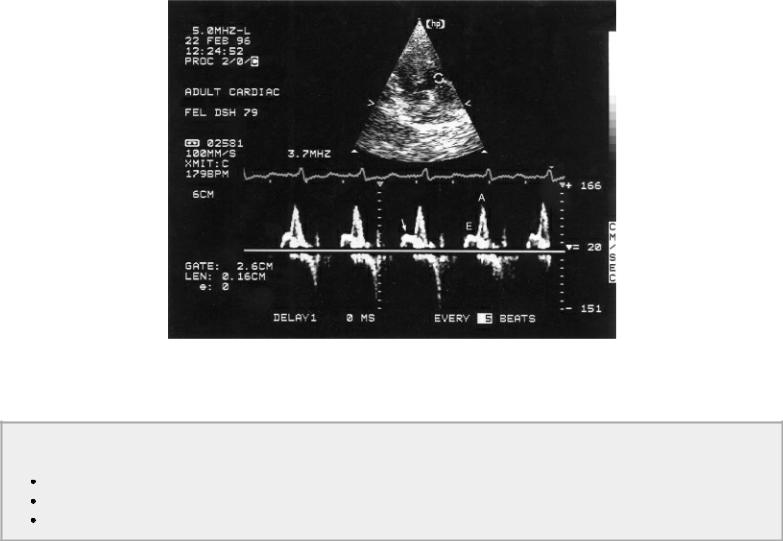
Figure 4.74 The heart rate in this cat is slow enough to separate the two phases of diastolic filling. The flow profile suggests impaired relaxation by the reduced E velocity, the high A velocity, and the slow deceleration time (arrow).
These changes in left ventricular filling secondary to impaired relaxation can be seen in patients with hypertrophic cardiomyopathy and hypertension.
Impaired Relaxation
Reverse E:A ratio
Slow MV deceleration
Long IVRT
Decreased peak E velocity occurs because left ventricular diastolic pressure does not decrease as much as in normal hearts. The smaller pressure gradient between the left atrium and left ventricle results in a lower peak E velocity. Deceleration time is also prolonged as the left ventricle takes longer to relax thus taking longer for ventricular and atrial pressures to equilibrate, and filling time is slower. Because the ventricle may not completely relax until late in diastole often the atrial contraction contributes more to ventricular filling than the early filling phase does. This results in a high peak A velocity and an E:A ratio of less than 1. Prolonged isovolumic relaxation time is also seen with impaired relaxation.
Decreased Compliance
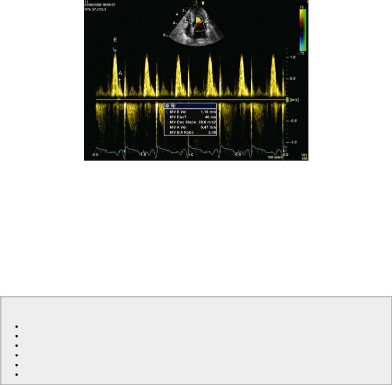
Restriction to left ventricular filling results in a short IVRT, increased E velocity, and decreased A velocity (Figure 4.75) (112,117,118,186,223,228,229). Left ventricular filling into a stiff noncompliant chamber produces a large increase in left ventricular pressure per unit volume. This kind of diastolic dysfunction is present in patients with restrictive, dilated, hypertrophic, or ischemic cardiomyopathy where high filling pressures are predominant. Most of ventricular filling occurs early in diastole and less occurs with atrial systole since pressure within the left ventricle elevates rapidly in early diastole, resulting in a high E:A ratio. Low A velocity may also be seen if atrial function is compromised. Deceleration times are typically reduced in these hearts secondary to rapid equalization of atrial and ventricular pressures.

Decreased Compliance
Short IVRT
High E:A ratio
Rapid MV deceleration
Figure 4.75 Restriction to ventricular filling results in high peak E velocities and decreased A velocities. Deceleration time is typically rapid in hearts with restrictive physiology as the atrial and ventricular pressured equalize rapidly (arrow).
Elevated Left Atrial Pressure
Elevated left atrial pressure seen with any of the cardiomyopathies results in higher E wave velocity and a more rapid equilibration between left ventricular and left atrial pressure that can be seen in the reduced E deceleration time (Figure 4.76). This is referred to as a restrictive filling pattern (121). There is an inverse relationship between deceleration time and left ventricular filling pressure in human patients with systolic myocardial failure (121,230). This parameter is considered to be one of the more specific indications of high left ventricular filling pressure, and studies in both man and dogs show a strong correlation between rapid E wave deceleration and mortality (121,231).
Figure 4.76 Elevated left atrial pressure, which can be seen with any of the cardiomyopathies, results in higher E wave velocity and rapid pressure equilibration between the left ventricle and atrium that can be seen in the reduced E deceleration time (MV DecT). This is referred to as a restrictive filling pattern.
The IVRT may be reduced or normal in hearts with restriction to filling since atrial pressures are higher. Isovolumic relaxation time decreases as left atrial pressure increases. Sinus tachycardia causes the E and A waves to fuse, which may result in a falsely shortened IRVT (121).
Pulmonary venous flow during systole is blunted in the presence of elevated left atrial pressure (Figure 4.77). Pulmonary vein systolic flow velocity may also be decreased in the presence of significant mitral regurgitation, atrial fibrillation, and severe left ventricular systolic failure.121 As left ventricular filling pressure increases, reverse flow during atrial contraction is accentuated. Velocity and duration are increased (Figure 4.78) (112). A pulmonary venous atrial reverse flow duration longer than transmitral atrial flow duration indicates decreased compliance as well as high left ventricular filling pressure (112).
Increased LA Pressure
High E:A ratio
Rapid MV deceleration
Decreased IVRT
Decreased pulmonary vein S
Increased pulmonary vein Ar duration and velocity
Increased E:Em
Figure 4.77 Here the S wave is blunted, the D wave has high velocity, and Ar is increased in duration (vertical lines) and velocity secondary to elevated LV filling pressure. S = pulmonary vein systolic flow, D = pulmonary vein diastolic flow, Ar = pulmonary vein reverse flow during atrial contraction.
Figure 4.78 As left ventricular filling pressure increases, reverse flow during atrial contraction (Ar) is accentuated. Ar duration is increased in this cat. This typically occurs before any changes in systolic
(S) and diastolic (D) flow are detected. S and D are normal here.
TDI diastolic motion is less preload dependent than conventional PW Doppler of transmitral valve flow in cats and people with hypertrophic heart disease (217,232). Tissue Doppler diastolic annular motion appears to be a good predictor of mortality and development of congestive heart failure in man (213). When both annular Sm and Em are lower than 3 cm/sec in man, it is predictive of significant mortality (233). This was an even more useful predictor when combined with a restrictive filling pattern (rapid E wave deceleration) and high E:Em ratios (233).
Diminished Em velocity then indicates impaired diastolic function (Figure 4.79) (217,234). Normal feline pulsed-wave TDI Em values should be greater than 7.2 cm/sec. In normal hearts, annular Em increases with exercise, increased preload, and increased transmitral pressure gradient. Hearts with increased left atrial pressure show increases in early transmitral flow velocity, and since Em decreases at all stages of diastolic failure, the E:Em (also written as E:E′) increases. E:Em in normal cats should be less than 8.07, and increases in this ratio are consistent with high left ventricular filling pressure
(217). The ratio of E:Em is a powerful negative prognostic indicator in man when its value exceeds 15 (213). An animal model of tachycardia-induced cardiomyopathy showed a progression of impaired relaxation pattern to a restrictive filling pattern as heart failure progressed. This means that transmitral E wave velocity was low, went through a pseudonormal phase, and progressed to a restrictive filling pattern. Em is reduced from early on in the progression of the disease process and remained low even as left atrial pressure increased and can be used to discriminate normal from pseudonormal transmitral flow velocities (112,235,236). When combined with transmitral flow early deceleration time (EDT), the more rapid the DT and the higher the E:Em the worse the prognosis (213). During treatment for congestive heart failure, it has been shown that persistence of a restrictive filling pattern (rapid mitral valve deceleration time, high mitral valve E) indicated a poorer prognosis as well. A reversible restrictive pattern is consistent with a better prognosis and longer survival time (213,237).
Normal Feline
E:Em < 8.07
 ↑ = increased LV filling pressure Em > .72 cm/sec
↓ = impaired diastolic function
Figure 4.79 Diminished E′ velocity indicates impaired diastolic function. In this cat, E′ is less than 7 cm/sec.
Pseudonormalization
Diastolic function is not a static thing, and various diseases create a continuum of changes in left ventricular preload and atrial pressure. A mitral valve flow profile may appear normal despite impaired diastolic function. This is referred to as pseudonormalization (Figure 4.80) (112,114,117,118). As left atrial pressure increases with advancing diastolic dysfunction, early transmitral flow velocity increases secondary to the increase in left atrial pressure. This changes the low transmitral valve E:A ratio back to normal (pseudonormal). As left atrial pressure increases even further, the restrictive filling pattern develops and the E:A ratio becomes significantly greater than 1.
During the time that left atrial pressures are just high enough to return the transmitral flow appearance to normal, isovolumic relaxation time also returns to normal. It does not take as long for left ventricular pressure to drop to left atrial pressure in this situation creating a pseudonormal isovolumic relaxation time period.
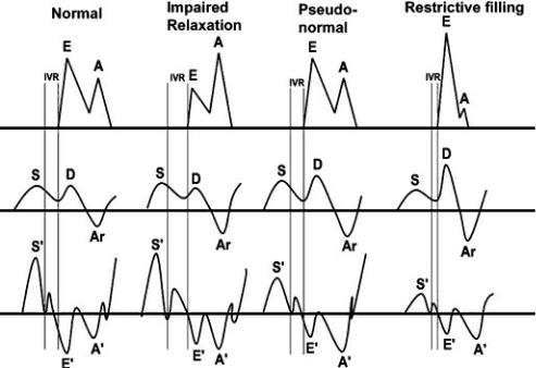
Figure 4.80 This diagram shows the progression from normal to impaired relaxation to pseudonormal to restrictive physiology of transmitral valve flow, pulmonary vein flow, isovolumic relaxation, and TDI motion. See text for more details. E = mitral valve E peak, A = mitral vale A peak, IVR = isovolumic relaxation, S = pulmonary vein systolic flow, D = pulmonary vein diastolic flow, Ar = pulmonary vein atrial reverse flow, S′ = myocardial systolic motion, E′ = myocardial early diastolic motion, A′ = late diastolic myocardial motion.
Normal from abnormal diastolic function can sometimes be differentiated by looking at pulmonary vein flow. Reversal of flow within the pulmonary veins is normally seen during atrial contraction. High velocity reversed flow, which encompasses the entire time period of atrial contraction, is seen when left ventricular diastolic pressure increases abnormally during atrial contraction regardless of mitral valve flow profiles (Figure 4.78). This may be used to evaluate diastolic function when heart rates are too high to separate the two phases of diastolic left ventricular inflow.
Valvular insufficiencies will alter the mitral inflow profiles. Significant aortic insufficiency will elevate left ventricular diastolic pressure quickly during early diastole. The gradient from left atrium to ventricle will decrease rapidly, and deceleration time will decrease. Moderate to severe mitral insufficiency typically produces a large pressure gradient between the left atrium and ventricle. Peak E velocity will increase accordingly (Figure 4.81). The presence of significant mitral insufficiency in hearts with hypertrophic or dilated cardiomyopathy may alter the expected flow profile. Increased atrial pressure for instance, would increase peak E inflow velocities by increasing the pressure gradient between the two chambers. A low left ventricular filling pressure secondary to decreased preload can intensify the changes seen with impaired relation simply due to lack of volume.
Figure 4.81 Peak E velocities increase for reasons other than impaired relaxation. Mitral insufficiency in this dog increases forward flow velocities (A) to 184 cm/sec.
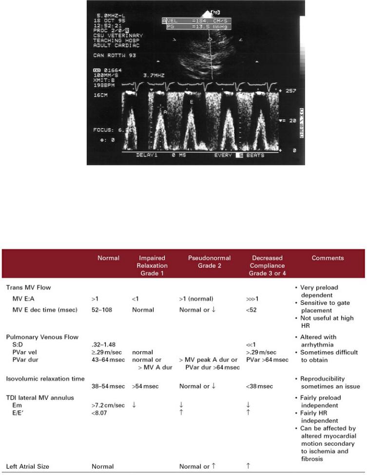
Grading of Diastolic Function
Diastolic function can be categorized into four grades. Altered transmitral and pulmonary vein flow, isovolumic relaxation time, and tissue Doppler velocity are used to assign the grade of diastolic failure (Table 4.3) (112,228).
Table 4.3 Grading of Diastolic Dysfunction
Modified from:
Kamp O. Advanced systolic and diastolic function: beyond the E and A wave. Sem Cardiothoracic and Vascular Anethesia

2006;10:63–65. (using feline reference values)
Lester SJ, Tajik AJ, Nishimura RA, et al. Unlocking the mysteries of diastolic function: deciphering the Rosetta Stone 10 years later. J Am Coll Cardiol 2008;51:679–689.
Guarracino F, Lapolla F, Danella A, et al. Reduced compliance of left ventricle. Minerva Anestesiol 2004;70:225–228.
Grade 1 diastolic failure is impaired or delayed ventricular relaxation. During this phase muscle relaxation is slower so early ventricular filling is impaired resulting in diminished transmitral valve E velocity and deceleration rate as well as a possible increased pulmonary vein S:D ratio. Diastolic filling of the atrium (which occurs at the same time as mitral E) is not optimal when early filling of the left ventricle is reduced.
Grade 2 diastolic dysfunction is present when left atrial pressure has increased enough to create the pseudonormalization phase. Mitral valve E:A and isovolumic relaxation time are normal. Pulmonary venous flow however shows increased Ar velocity and duration. Tissue Doppler E:Em is increased during this time period as it reflects the increase in left atrial pressure.
Diastolic Dysfunction
Stage I
Delayed relaxation
Compliance normal
LV filling pressure normal
Stage II
Pseudonormal
Impaired relaxation
Decreased compliance
LV filling pressure increased
Stage III and IV
Restrictive physiology
Severely impaired relaxation
Severely decreased compliance
Very high LV filling pressure
Diastolic dysfunction that has progressed to the stage where left atrial pressure is significantly increased and left ventricular filling pressure is high is Grade 3 diastolic dysfunction. Here transmitral E:A is significantly higher than 1.0 (often greater than 2.0), pulmonary vein Ar is increased in duration and velocity, pulmonary vein D is significantly increased, and S is significantly reduced secondary to the elevated left atrial pressure. Tissue Doppler E:Em remains elevated. Irreversible diastolic dysfunction is Grade 4.
Hemodynamic Information Obtained From
Echocardiographic Exams
Doppler Hemodynamic Information
Doppler echocardiography has created what is referred to as the non-invasive cardiac catheterization. The peak velocity of valvular regurgitations and shunts are dependent upon the pressure difference
between the two chambers or vessels involved. When a pressure gradient is calculated, it means that the pressure within the driving chamber or vessel is that much higher than the pressure within the receiving chamber or vessel. The pressure in the receiving chamber is estimated and added to the calculated gradient in order to determine pressure within the driving chamber. These are of course based on estimates of pressure within the receiving chamber, and some error is inherent within the application. As the following applications are described, ways to estimate atrial and ventricular pressure will be discussed.
Pressure Gradients
This is probably the most common application of Doppler echocardiography in veterinary medicine. The physical principle of Conservation of Energy is the basis of the Bernoulli equation, which is used to calculate the pressure gradient between two areas of the heart (99,186). The principle states that when a constant volume of blood flows through a narrowed area, its velocity must increase by an amount equal to the pressure drop (Figure 4.82). When a constant volume of blood is moved through an orifice or vessel, the pressure increase proximal to the obstruction creates a proportional increase in blood velocity through the obstruction. The greater the degree of obstruction between the driving chamber and the receiving chamber or vessel the greater the pressure differential and the higher the velocity of blood will be. The Bernoulli equation (Equation 4.30) is as follows:
Equation 4.30 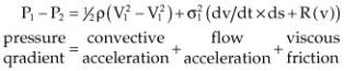
Figure 4.82 When a constant volume of fluid flows through a narrowed vessel or tube its velocity must increase. This is seen in everyday life when a thumb is placed over the end of a hose in order to increase the velocity and pressure of the spray.

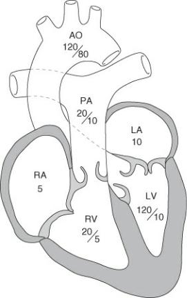
The forces of viscous friction and flow acceleration are negligible in most causes of heart disease. The value of 1/2 ρ, the mass density of blood, is about 4, so the Bernoulli equation is simplified as follows (Equation 4.31):
Equation 4.31 
where ΔP = the pressure gradient, V1 = blood velocity proximal to the obstruction or orifice, and V2 = blood velocity distal to the obstruction or orifice. The velocity is measured in meters per second and the pressure gradient is mm mercury (Hg).
Modified Bernoulli Equation
PG = 4V2
For example, if a PW sample gate placed at a subvalvular aortic stenosis within the left ventricular outflow tract produces a velocity of 1.2 m/sec, and velocity distal to the obstruction in the aorta is 3 m/sec, the following pressure gradient is calculated:
ΔP = 4(32 − 1.22) ΔP = 30.2 mm Hg
Most normal flows within the heart are close to 1 m/sec, so the effect of V1 is negligible and an even more simplified form of the equation (Equation 4.32) is usually used:
Equation 4.32 
This is called the simplified Bernoulli equation. Using the previous example, 4(32) = 36 mm Hg. Therefore, using the modified Bernoulli equation usually overestimates the pressure gradient to a small degree.
Mean pressure gradients calculated from Doppler flow profiles can be determined by calculation packages within the ultrasound machine. The flow profile is traced and digitized. An arithmetic mean gradient is calculated that has a high correlation with catheterization-derived mean gradients. Mean and peak pressure gradient calculation is shown in Figure 4.83.
Figure 4.83 (A) The peak velocity of 569 cm/sec is inserted into the modified Bernoulli equation and a pressure gradient of 130 mm Hg is calculated. (B) Tracing the flow velocity profile yields both maximum velocity (Max V) 419 cm/sec, mean velocity (Mean V) 287 cm/sec, velocity time integral (VTI) 47.4 cm, the peak pressure gradient (Max PG) 70.2 mm Hg, and the mean pressure gradient (Mean PG) 38.3 mm Hg. Dynamic outflow obstruction is evident by the late peaking flow profile (arrow).
Blood volume, tunnel lesions, and blood viscosity all place limitations to the application of the Bernoulli equation (99,186,187). Since flow velocity is also dependent upon the volume of blood moving through a vessel or orifice, pressure gradient calculations will be inaccurate when there is a high flow state (V1 will be elevated). Such conditions will exist when there is severe valvular insufficiency through a valve or through a stenotic area (i.e., aortic insufficiency and aortic stenosis, a coexisting shunt, anemia, or sepsis). In the presence of conduit type of lesions as in tunnel subvalvular aortic stenosis, the Bernoulli equation will overestimate the pressure gradient since the effects of friction are no longer insignificant. Pressure gradients may also be overestimated when the viscosity of blood is decreased. Increased blood viscosity may underestimate the pressure gradient. Since the sample site for measuring aortic flow velocity proximal to an aortic stenotic lesion within the left ventricular outflow tract is often very deep, the signal may alias even with low frequency transducers. It would not be possible to determine V1 accurately, and the calculated pressure gradient will be higher than it actually is.

Pressure gradients not accurate when:
The intercept angle is large.
Conduit-type obstruction is present.
There is valvular insufficiency at the obstruction.
V1 is not negligible.
Although there is very good correlation between catheterand Doppler-derived pressure gradients, there is a difference in the way the gradients are measured, which makes it appear that the Dopplerderived gradient overestimates the gradient when compared to gradients derived during cardiac catheterization (99,186,238). Doppler-derived pressure gradients calculate maximal instantaneous pressure differentials across the stenotic lesion while catheterization-derived pressure gradients are peak-to-peak differentials (Figure 4.84). Peak-to-peak pressure gradients in aortic stenosis for example, are determined by calculating the difference between maximal left ventricular pressure and maximal aortic pressure. These two pressures do not occur at the same time. Doppler-derived pressure gradients are calculated from the maximal instantaneous pressure difference between ventricular and aortic pressure. This creates a discrepancy between invasiveversus noninvasive-derived gradients since instantaneous gradients may be as much as 30 to 40% higher than peak-to-peak gradients. The more severe the stenosis, the closer peak-to-peak and instantaneous pressures are, since the highest left ventricular pressures are generated later in systole. The arithmetic mean gradient calculated from Doppler flow profiles has a high correlation with catheterization-derived mean gradients.
Figure 4.84 (A) Pressure gradients (PG) derived from catheterization are peak to peak (P to P). Peak ventricular pressure is compared to peak aortic pressure and the difference reflects the peak-to-peak pressure gradient. (B) Doppler echocardiography derives instantaneous pressure gradients (IPG) by determining the maximum difference in pressure at any given instant during ejection. This is typically higher than peak-to-peak calculations.
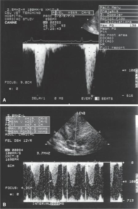
In order to fully apply Doppler echocardiography, estimates of intracardiac pressure are necessary. Figure 4.85 shows typical pressures within the cardiac chambers and great vessels. Unless stated otherwise, these are the values that will be used in any exercises and examples presented in this book. Disease processes may change these pressures somewhat, but unless invasive procedures are available, they are a good estimate, and using these representative pressures will not diminish the usefulness of Doppler-derived information in most applications.
Figure 4.85 Typical intracardiac pressures are displayed in this diagram of the heart’s chambers and vessels. AO = aorta, PA = pulmonary artery, LA = left atrium, RA = right atrium, RV = right ventricle, LV = left ventricle.
Intracardiac pressure determination from Doppler flows and pressure gradients are based on estimates of pressure within the receiving chamber or vessel, and some error is inherent within the application. The pressure gradient can always be used as an “at least” pressure. For example, if the pressure gradient from left ventricle to left atrium is calculated as 130 mm Hg, the left ventricular pressure is “at least 130 mm Hg” regardless of what the left atrial pressures are.
The simplified Bernoulli equation is used in many applications. It is applied to stenotic lesions involving the great vessels or atrioventricular valves, ventricular and atrial septal defects, and intracardiac pressure determination by regurgitant jets. Mathematical software packages within the ultrasound equipment will calculate pressure gradients after peak velocity through the stenosis, shunt, or leak is identified and mean pressure gradient when the FVI is traced.
An example of a pressure gradient calculated from a dog with subvalvular aortic stenosis is seen in Figure 4.83. The pressure gradient of 130 mm Hg means that pressure within the left ventricle is 130 mm Hg higher than pressure beyond the obstruction in the aorta. Exercises involving pressure gradient calculations across stenotic lesions are found at the end of this chapter.
Systolic Left Ventricular and Systemic Pressures
Systolic pressure within the left ventricle is fairly equal to peripheral systolic blood pressure in the absence of left ventricular outflow obstruction. The driving pressure of a mitral regurgitant jet therefore would equal both ventricular systolic pressure and systolic blood pressure (239). Since left ventricular pressure is typically at least 100 to 110 mm Hg, and left atrial pressure is usually less than 10 mm Hg, a pressure gradient close to 100 is expected when the Bernoulli equation is applied to the peak velocity of a mitral regurgitant jet. This means that velocities of close to 5 m/sec should be recorded from a mitral regurgitant jet (4 × 52 = 100).
Left atrial pressure can be estimated and added to the pressure gradient in order to calculate left
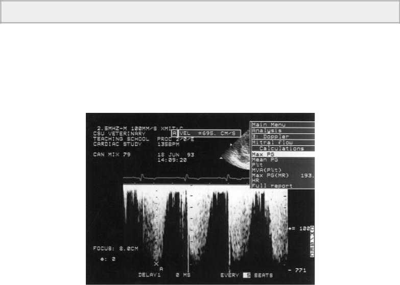
ventricular pressure, but even if left atrial pressure is not estimated and assumed to be zero, left ventricular and systemic pressures are at least equal to the pressure gradient. As systemic pressure increases the driving pressure from left ventricle to atrium will also increase, and peak velocity will increase accordingly (Figure 4.86). An animal with a regurgitant jet velocity of 6.8 m/sec, (4 × 6.82 = 185), would have systolic systemic pressures of at least 185 mm Hg. Exercises at the end of the chapter apply this principle. Many cases of systemic hypertension have been found inadvertently by interrogating mitral regurgitant jets. Often Doppler assessment of high blood pressure is easier to obtain than good peripheral measurements of blood pressure especially in smaller animals. A “white coat” effect similar to that seen in people may be seen in animals, and pressure may only be elevated secondary to the stress of the clinical environment. Severe mitral regurgitation with a significant degree of flow acceleration proximal to the mitral valve will overestimate the pressure gradient because V1 is no longer negligible (99,186,187).
Use mitral or tricuspid insufficiencies to double check a pulmonic or aortic pressure gradient.
Figure 4.86 Peak velocities from mitral regurgitant jets can be used to determine the systolic driving pressure of the left ventricle. Here a peak velocity of 695 cm/sec is inserted into the Bernoulli equation to yield a calculated pressure gradient of 193 mm Hg. Left ventricular pressure is at least 193 mm Hg. In the absence of aortic stenosis this is also a reflection of systemic pressure. In the presence of aortic stenosis, it suggests a pressure gradient of approximately 73 across the obstruction since ventricular pressure is at least 193 and aortic pressure is approximately 120.
Systolic Right Ventricular and Pulmonary Pressures
These same principles are applied to the right side of the heart and have been studied in the dog (240). Right ventricular systolic pressure approximates pulmonary artery systolic pressure in the normal heart. Therefore, the driving pressure behind a tricuspid regurgitant jet will equal both right ventricular systolic pressures and pulmonary systolic pressure in the absence of pulmonic stenosis (187). Right ventricular and pulmonary systolic pressures are typically about 20 to 25 mm Hg, and

right atrial pressure is normally less than 5 mm Hg. A normal pressure gradient between the right ventricle and atrium would be about 15 to 20 mm Hg. If a tricuspid regurgitant jet with a velocity of 2.3 m/sec is recorded, the calculated pressure gradient is 21 mm Hg, indicative of normal right ventricular and pulmonary systolic pressures. Regurgitant jets with higher velocities are suggestive of elevated right ventricular and pulmonary artery systolic pressures (Figure 4.87). Exercises applying the Bernoulli equation to tricuspid insufficiency may be found at the end of the chapter.
Figure 4.87 Peak velocities from tricuspid regurgitant jets are used to determine right ventricular systolic pressures. Here a velocity of 455 cm/sec and a pressure gradient of 82.8 suggest right ventricular systolic pressures are at least 83 mm Hg. In the absence of pulmonic stenosis, this is a reflection of pulmonary systolic pressures. In the presence of pulmonic stenosis, it suggests a pressure gradient of approximately 63 across the obstruction since ventricular pressures are at least 83 and pulmonary pressures are approximately 20.
When aortic stenosis and mitral insufficiency are both present, the left ventricular pressure affects both the aortic flow velocity and the mitral regurgitant velocity (Figure 4.85). A pressure gradient of 100 mm Hg calculated from the aortic flow profile in the presence of aortic stenosis tells us that left ventricular pressure is 100 mm Hg greater than systemic pressure. If systolic blood pressure is 100 mm Hg then left ventricular pressure is approximately 200 mm Hg. Doppler interrogation of mitral insufficiency should show a peak velocity of about 7 m/sec if aortic flow profiles were accurately recorded (4 × 72 = 196). This can be used to double check the Doppler results. Mitral regurgitation can often be used to verify or help determine a left ventricular to aorta pressure gradient in the presence of subvalvular or valvular aortic stenosis. If there is a discrepancy between the two determinations of left ventricular pressure then the highest estimate should be used since Doppler rarely overestimates a pressure gradient but often underestimates a gradient when the interrogation angle with respect to flow becomes large. For example, with a systolic blood pressure of 120, if a gradient of 60 is obtained for a subvalvular aortic stenosis (suggesting ventricular pressure of approximately 180 mm Hg), and a gradient of 220 is obtained from a small mitral regurgitant jet (suggesting left ventricular pressure of approximately 220 mm Hg), then the pressure gradient across the aortic valve is underestimated and
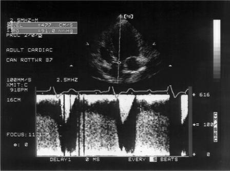
should be closer to and at least 100 mm Hg (220–120).
The same process can be applied to right-sided pressure calculations when both tricuspid insufficiency and pulmonary stenosis is present. The pressure gradient measured from the tricuspid regurgitant jet may be used to determine or verify the severity of the pulmonic stenosis. Applications of this can be found at the end of the chapter.
Diastolic Systemic Pressure
Diastolic systemic pressures can be determined noninvasively if aortic insufficiency is present. Peak velocity of the aortic insufficiency can be used to determine the pressure gradient between the aorta and left ventricle during diastole. A normal diastolic systemic pressure of 60 and a normal left ventricular end diastolic pressure of 10 yield a pressure gradient of 50. A peak aortic insufficiency velocity of 3.5 m/sec would suggest normal systemic diastolic pressure (4 × 3.52 = 49). As diastolic systemic pressure increases with hypertension, the driving pressure into the left ventricle becomes greater, and higher peak aortic regurgitant velocity is expected (Figure 4.88). Aortic insufficiency with a peak velocity of 4.8 m/sec suggests diastolic blood pressure of at least 92 mm Hg (4 × 4.82 = 92). Exercises for pressure gradient calculation with aortic insufficiency are at the end of the chapter. As with systolic pressure estimation, animals do display a “white coat effect,” and blood pressure may only be temporarily elevated due to the clinical environment.
Figure 4.88 A velocity of 477 cm/sec and a pressure gradient of 91 mm Hg are calculated from this aortic insufficiency flow profile. This implies that diastolic systemic pressures are at least 91 mm Hg.
Diastolic Pulmonary Pressure
Pulmonary hypertension elevates both systolic and diastolic pressures. Since a large number of normal animals have pulmonary insufficiency, this jet may be used to determine pulmonary diastolic pressure. The presence of elevated diastolic pulmonary pressure confirms the presence of pulmonary hypertension even if systolic pulmonary pressure cannot be derived from a tricuspid regurgitant jet. Since normal pulmonary diastolic pressure is approximately 10 to 15 mm Hg, and right ventricular
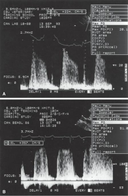
diastolic pressure is less than 5 mm Hg, a pressure gradient of about 10 to 15 mm Hg is expected in the normal heart from the pulmonary artery to the right ventricle. Pulmonic insufficiency jets should have velocities no greater than 2 to 2.5 m/sec in animals with normal pulmonary pressures (4[22] = 16) (Figure 4.89). See exercises at the end of the chapter to apply these pressure calculations.
Figure 4.89 (A) A velocity of 224 cm/sec and a pressure gradient of 20.1 mm Hg calculated from this pulmonic insufficiency flow profile suggest normal mean pulmonary artery pressure of about 25 mm Hg. (Add the estimated right ventricular diastolic pressures of about 5 mm Hg to the pressure gradient of 20.) (B) A pressure gradient of 51 on this pulmonic insufficiency flow profile is high and indicative of pulmonary hypertension.
Peak early diastolic regurgitant pressure gradient represents mean pulmonary artery pressure. The pressure gradient obtained at end diastole is used to calculate end diastolic pulmonary artery pressure (Figure 4.90). Adding an estimated right ventricular end diastolic pressure to the end diastolic
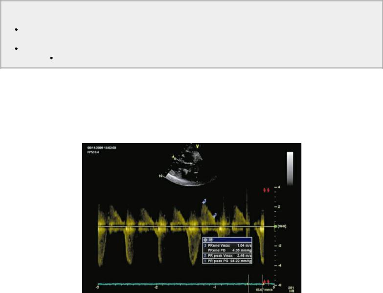
pressure gradient obtained from the pulmonary regurgitant jet represents the end diastolic pressure in the pulmonary artery. Right ventricular diastolic pressure is estimated from vena cava collapse during respiration. See Chapter 5 for a discussion on vena cava collapse and estimating right atrial pressure.
Pulmonary Insufficiency
Peak early pressure gradient
 = mean PA pressure End diastolic pressure gradient
= pulmonary artery diastolic pressure
Figure 4.90 Peak early diastolic regurgitant pressure gradient represents mean pulmonary artery pressure. The pressure gradient obtained at end diastole is used to calculate end diastolic pulmonary artery pressure. PRend Vmax = pulmonary regurgitation end diastolic velocity, PRend PG = pressure gradient at end diastole, PR peak Vmax = peak pulmonary regurgitant velocity early is diastole, PR peak PG = pressure gradient early in diastole.
Regurgitant Fraction
Flow through the mitral annulus is equal to flow out the aorta in a normal heart as is flow through the mitral and tricuspid valves and flow through the aortic and pulmonary valves and flow through the tricuspid and pulmonary valves. This of course is true over the course of several cardiac cycles since there are variations in stroke volume related to heart rate and respiration on a beat-to-beat basis. Only when there are insufficiencies or shunts will there be more volume flowing through one valve than another. In the case of mitral insufficiency, flow through the mitral valve will be greater than flow through the aortic valve. The regurgitant volume plus the normal forward stroke volume moves past the mitral valve and then as the normal forward stroke volume goes through the aorta, the regurgitant volume flows back into the left atrium (187). Based on this, regurgitant fractions (RF) can be calculated by applying Equation 4.33:
Equation 4.33 

where SV = stroke volume, which is calculated using Equations 4.25, 4.26, and 4.27.
Limitations to this application include inaccuracies in area calculations for the aorta and mitral annuluses as well as the fact that the stroke volume at each valve is not measured at the same cardiac cycle. Measure five or more cardiac cycles for area measurements (Equation 4.25) in order to eliminate as much technical error as possible as well as beat-to-beat flow differences. As with shunt ratios in the next section, no one piece of information should be used to assess the severity of a cardiac lesion. All the information available including the degree of volume overload, function, flow velocities, and profiles as well as the clinical picture should be evaluated. Regurgitant fractions are just one way of assessing regurgitation, and this area of echocardiography needs further investigation in veterinary medicine.
Shunt Ratios
Analysis of cardiac shunts should involve analysis of the shunt pathway. Only the chambers and vessels of the heart that are in the pathway will show enlargement or increased flow volume. A ventricular septal defect therefore has increased volume within the left ventricle, right ventricle, pulmonary artery, and left atrium. The right atrium and aorta never see the shunted volume. With atrial septal defects the shunt volume flows through the left atrium, right atrium, right ventricle, and pulmonary artery. The left ventricle and aorta never see the shunt volume. Patent ductus arteriosus (PDA) volume overloads the pulmonary artery, the left atrium, the left ventricle, and ascending aorta. The right side of the heart is not affected by a typical leftto right-flowing PDA.
Based on the flow pathways then the severity of a ventricular septal defect, atrial septal defect, or PDA can be assessed by analyzing flow through an area that should not see the shunted volume versus an area that does. This is done by determining Qp/Qs, where Qp = pulmonary flow and Qs = systemic flow. The greater the volume of blood shunting across a ventricular septal defect for instance the greater the amount of flow out the pulmonary artery versus the aorta where the shunted blood never passes. Calculation of a shunt ratio for ventricular septal defect or atrial septal defect can be done by applying Equation 4.34:
Equation 4.34 
where PAsv = pulmonary artery stroke volume and AOsv = aortic stroke volume. Stroke volume is calculated using Equations 4.25, 4.26, and 4.27.
Qp:Qs
= shunt ratio for VSD and ASD
Qs:Qp
= shunt ratio for PDA
Patent ductus arteriosus is different in that the increased flow is seen in the ascending aorta, and normal stroke volume is seen in the pulmonary artery. Its shunt ratio (Equation 4.35) is therefore calculated as follows:
Equation 4.35 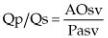
As with regurgitant fractions there are limitations to this technique. The most limiting factor is again area calculation for the aorta and pulmonary artery. Shunt severity should never be assessed by

one method alone. The entire exam should be considered including cardiac size, flow velocities, as well as the clinical picture.
Pressure Half-Time
Aortic Regurgitation
The effects of aortic insufficiency on left ventricular diastolic pressure can be assessed from the shape of the aortic regurgitant flow profile (99,186,187,241). At any point during diastole, the instantaneous pressure difference between the aorta and left ventricle is reflected upon the regurgitant jet flow profile. When aortic insufficiency is severe, there will be a rapid decline in aortic diastolic pressure because of runoff into the left ventricle, and there will be a dramatic increase in left ventricular pressures. Both of these factors produce a rapid decline in regurgitant velocity as the driving pressure into the left ventricle declines and the receiving pressure increases creating less of a pressure gradient. The flow profile becomes triangular in shape as opposed to the flat plateau-shaped flow profiles seen in mild aortic insufficiency (Figure 4.91). Mild aortic insufficiency does not elevate left ventricular diastolic pressure significantly and neither does it decrease aortic diastolic pressures dramatically. The result is a flow profile that is plateau shaped because the pressure gradient remains similar throughout diastole (Figure 4.92).
Pressure Half-Times
= time for peak velocity to decline by half
Aortic Regurgitation
Hemodynamically insignificant
PHT = long
PHT = plateau shaped
Hemodynamically significant
PHT = short
PHT = steep slope
Figure 4.91 The rapid deceleration of this aortic insufficiency flow profile suggests that left ventricular and aortic diastolic pressures are equilibrating rapidly. PHT = pressure half time.
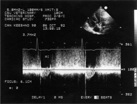
Figure 4.92 Mild to moderate aortic insufficiencies that do not increase ventricular diastolic pressures are plateau shaped.
The rapid decline in aortic regurgitant velocity can be measured, and the measurement is referred to as the diastolic pressure half-time. This is the time it takes for the peak gradient (not velocity) to decrease by half. The measurement is made by extending the deceleration slope to the baseline and measuring the deceleration time (Figure 4.93). This deceleration time is multiplied by .29. The calculations are performed by the equipment automatically. There are no standards for measurement of diastolic half-times in animals, and even in man, there are problems in applying half-time measurements. Diastolic half-times less than 300 m/sec are suggestive of hemodynamically significant aortic regurgitation (186,241). The measurement cannot separate groups of patients into mild, moderate, and severe insufficiency consistently however, and there is much overlap. Part of the problem may lie in the fact that several flows affect aortic and ventricular pressures including transmitral flow into the ventricle while the aortic valve is leaking, and forward flow into the system at the same time as the regurgitant flow. Nevertheless, a subjective assessment of flow profile is easy enough to apply, and significant aortic insufficiency as well as a rapid increase in left ventricular diastolic pressure can be assumed from a sharp decline in aortic regurgitant velocity during diastole.
Figure 4.93 The rapid decline in aortic regurgitant velocity can be measured and the measurement is referred to as the diastolic pressure half-time. This is the time it takes for the peak gradient (not velocity) to decrease by half. AR = aortic regurgitation, Vmax = maximum velocity, PG = pressure gradient, PHT = pressure half-time, Dec = deceleration.
Mitral and Tricuspid Stenosis
The severity of mitral or tricuspid stenosis correlates directly with pressure half-time. The longer the pressure half-time the more severe the stenosis (Figure 4.94) (242–245). The velocity across the stenosis is directly dependent upon left ventricular pressures. This is in contrast to the pressure halftimes seen in aortic and pulmonary regurgitation. The reduced slope reflects delayed normal early diastolic closure because of a persistent pressure differential between the left atrium and left ventricle. Normal mitral valve pressure half-time in the dog are 29 ± 8 m/sec (<50 m/sec) and are reported to be less than 30 m/sec in the cat. Normally during early ventricular filling, the left ventricular pressure rises and left atrial pressure decreases resulting in a rapid deceleration of the E peak on transmitral flow profiles when the pressure gradient between the two chambers rapidly equalizes. With mitral or tricuspid stenosis, the more severe the restriction to ventricular inflow the longer the pressure gradient is maintained between the two chambers and the slower the decline of the MV or TV E peak during early diastolic filling.
Figure 4.94 The severity of mitral or tricuspid stenosis correlates directly with pressure half-time (PHT). The longer the PHT, the more severe the stenosis. PHT = pressure half-time, MV = mitral valve, MVA = mitral valve area.

M-Mode Hemodynamic Information
Doppler echocardiography provides direct assessment of blood flow within the heart and is the primary method used to assess the hemodynamics of flow within the ventricles and atria. This does not diminish the valuable hemodynamic information that can be derived from two-dimensional and M-mode images. Even without the quantitative information available through Doppler, the following M-mode features can provide very definite information about flow within the heart.
Aortic Valve Motion
Aortic valve motion on M-mode images reflects cardiac output. Normally the aortic valve opens rapidly, and the leaflets parallel each other as they lie along the aortic wall during systole. The end of systole produces rapid closure of these cusps. M-mode images that show normal opening at the onset of systole, but then show gradual closure of the cusps throughout systole, suggest that blood flowing through the aorta is decreasing as systole progresses (Figure 4.95) (246). This is typically seen when systolic function is impaired and cardiac output cannot be maintained throughout systole. It is also a frequent finding in patients with severe mitral insufficiency and low output failure where blood flows into the low pressure left atrium as opposed to the high-pressure aorta.
Figure 4.95 An aortic valve that displays gradual closure of the valve (arrows) implies a reduction in forward flow throughout systole. Here are three examples of gradual closure. These animals had (A) dilated cardiomyopathy, (B) mitral insufficiency, and (C) dilated cardiomyopathy. AO = aorta, LA = left atrium.
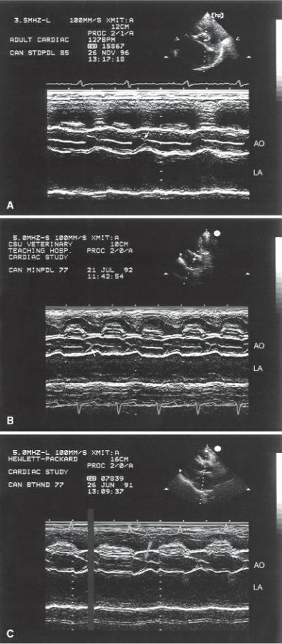
Systolic aortic valve fluttering is often seen in diseases that create turbulent and rapid blood flow through the aorta as in subvalvular aortic stenosis or hypertrophic obstructive cardiomyopathy (Figure 4.96). When the aortic valve exhibits midsystolic closure or notching, it is an indication that flow has been abruptly reduced at that point in time (Figure 4.97) (247,248). This is usually seen with dynamic
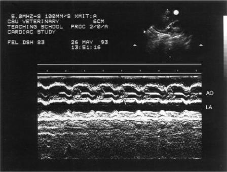
obstructions to left ventricular outflow. Dynamic obstruction including subvalvular muscular obstruction that increases with contraction of the ventricular septum and systolic anterior mitral valve motion. Systolic aortic valve closure can also be seen with discrete aortic stenosis. It is typically seen earlier in the systolic time period however (248). This is not specific to obstructive disease, but it is rarely seen otherwise. It has been reported with mitral insufficiency, ventricular septal defect, aortic root dilation and dilated cardiomyopathy (248,249).
Figure 4.96 The rapid velocity of blood as it flows past an obstruction can cause systolic flutter of the aortic valve (arrow). AO = aorta, LA = left atrium.
Figure 4.97 Varying degrees and displays of early or mid-systolic closure (arrows) of the aortic valve are seen in Figures A through E. This motion is usually seen with subvalvular obstruction to aortic outflow in the dog and cat as flow is disrupted. AO = aorta, LA = left atrium.
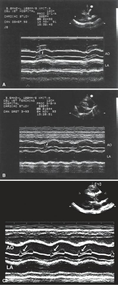
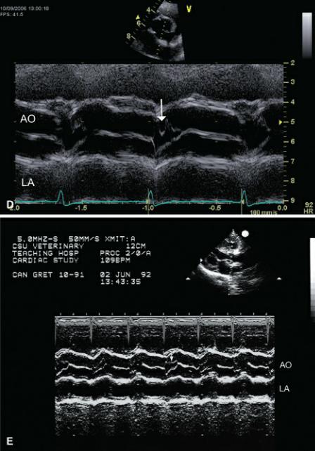
Mitral Valve Motion
As discussed previously, there are two phases to left ventricular filling, a rapid passive filling phase, and a slower active phase secondary to atrial contraction. These two phases create the classic “M” shape of the mitral valve. A reduction in deceleration after peak E velocity has been reached is generally associated with a decrease in the rate of filling secondary to delayed ventricular relaxation or increased stiffness of the ventricular walls (Figure 4.98). This is not a specific finding and may occasionally be seen in normal hearts and in patients with pulmonary hypertension or other volume contracted states.
Figure 4.98 A reduced deceleration slope (arrow) to the mitral valve on M-mode images is usually associated with reduced ventricular compliance. The large arrow shows mitral valve prolapse.

Patients in which left ventricular filling pressure is high will show early rapid closure of the mitral valve (250–252). Typically the valve closes shortly after the beginning of the QRS complex. In early closure the C point may occur before the QRS complex. This is a subtle and nonspecific finding. Mitral valve closure may also be delayed producing what is called the “B” bump (Figure 4.99) (253– 255). This is also found with elevated left ventricular pressure and is thought by some to reflect diastolic mitral insufficiency secondary to the high filling pressure (256,257). This is a normal finding in many horses and typically disappears with exercise.
Figure 4.99 Delayed closure of the mitral valve (arrows) on these two figures indicates decreased ventricular compliance and increased stiffness to the ventricle. The delay is referred to as a B bump. RV = right ventricle, LV = left ventricle.

The E point to septal separation as discussed earlier correlates significantly with left ventricular ejection fraction (Figure 4.38) (84–86). The EPSS may also be affected by aortic insufficiency however, as the regurgitant jet within the left ventricular outflow tract prevents the valve from moving completely up toward the septum (Figure 4.100). The turbulence associated with aortic insufficiency will also create vibration of the mitral valve during diastole. This vibration may sometimes also be seen on the interventricular septum. The worse the aortic insufficiency the greater the EPSS, the coarser the mitral valve diastolic flutter, and the more abnormal the “M” appears.
Figure 4.100 Diastolic flutter is often seen with aortic regurgitation, and the E point to septal separation (EPSS) may be larger than normal. (A) Here, a horse with severe aortic regurgitation shows diastolic mitral valve flutter and an increased EPSS (arrow). (B) This shows diastolic mitral valve flutter (arrows) with a normal EPSS. (C) A large EPSS and diastolic mitral valve flutter (arrows) are seen here. RV = right ventricle, LV = left ventricle.

Mitral valve motion also changes with left ventricular outflow obstruction. The mitral valve moves up toward the septum and left ventricular outflow tract creating what is referred to as systolic anterior
mitral (SAM) valve motion (Figure 4.101) Several theories exist for the underlying cause of SAM. High velocity flow within an outflow tract narrowed by a hypertrophied septum may create a Venturi effect and tends to pull one or both mitral valve leaflets along with it toward the septum (258–260). The presence of abnormal ventricular architecture and papillary muscle misalignment may allow the anterior or posterior mitral valve to be pushed into the outflow tract during systole (258,260–262). Alignment of the subauricular papillary muscle into the middle of a hypertrophic ventricular chamber may also play a role in the development of SAM (263). Refer to Chapter 7 for more detail on SAM in the presence of hypertrophic cardiomyopathy. This motion in itself adds to the obstruction to flow as the leaflet is pulled into the outflow tract (264–268). The greater the upward motion and the more apposition the mitral leaflet has with the septum during systole, the greater the degree of obstruction. This is a sensitive finding in moderate to severe dynamic left ventricular outflow obstruction but may occasionally be seen in hearts with transposition of the great vessels, coronary artery disease, systemic hypertension, discrete aortic stenosis, tunnel aortic stenosis, and mitral stenosis (269–273).There are other less frequently reported incidences of SAM in patients with glycogen storage diseases, and Friedreich’s ataxia (274,275).
Figure 4.101 Systolic anterior motion (SAM) of the mitral valve may be seen with outflow obstruction, abnormal papillary muscle alignment or with increased flow velocity through the left ventricular outflow tract. (A) Real-time images show the mitral valve pulled up into the outflow tract during systole (arrow). Figures B through E show varying degrees of SAM in (B) a dog, (C) a cat, (D) a dog, and (E) a cat. RV = right ventricle, LV = left ventricle, AO = aorta, LA left atrium.
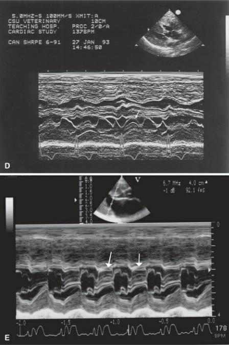
Left Ventricular Wall
Restriction to ventricular filling as seen with restrictive pericarditis or restrictive cardiomyopathy is difficult to assess with M-mode or even two-dimensional images. In some cases, however there are alterations in left ventricular wall motion. Normally the left ventricle gradually fills and there is concomitant downward motion of the free wall during diastole. With restriction to filling, left ventricular wall motion is flat with no increase in ventricular dimension toward the latter part of diastole since filling is impaired (276). This is a subtle and not a very sensitive finding but when present is specific.
Interventricular Septum
Animals with right-sided pressure or volume overload show paradoxical and flattened septal motion (277–279). This motion appears to be specific for right-sided disease and is not seen in left-sided cardiac disease. Normally the septum moves downward during early systole with peak downward
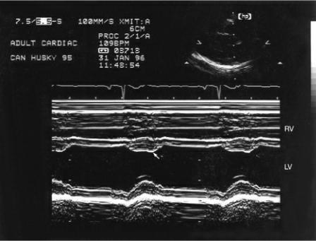
motion occurring just before peak upward motion of the left ventricular free wall. The septum then begins to move upward again at the end of systole and may show a diastolic dip (Figure 4.102). The dip may be associated with early left ventricular filling or when right ventricular filling occurs slightly before left ventricular filling (277).
Figure 4.102 A diastolic dip (arrow) is seen on many M-mode images of the left ventricle. It is thought to be related to early diastolic filling. RV = right ventricle, LV = left ventricle.
In the presence of right ventricular systolic pressure overload, right ventricular systole lengthens, despite a possibly shortened ejection time. This lengthened systolic period extends into the time when the left ventricle starts to relax. As a result the interventricular septum moves down to the left early in diastole. With the onset of left ventricular contraction, left ventricular pressure becomes higher than right-sided pressure again, and the septal motion moves to the right. This results in paradoxical septal motion. When there is also elevated right ventricular filling pressure, then the septum remains deviated toward the left throughout the diastolic time period with upward motion occurring only at peak left ventricular contraction (Figure 4.103) (170).
Figure 4.103 Paradoxical septal motion (PSM) is seen secondary to right ventricular volume and/or pressure overload. Figures A through D show varying degrees of PSM (arrows). RV = right ventricle, LV = left ventricle.
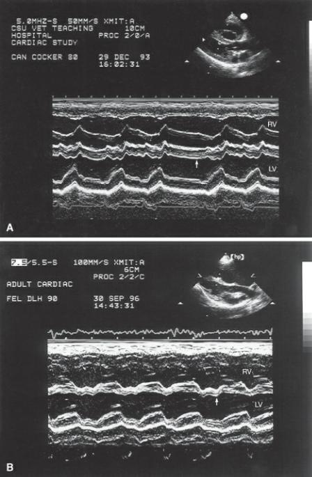
The right-sided volume overload must be moderate to severe before paradoxical septal motion is seen (277). Animals with right-sided volume overload, which elevates RV diastolic pressure but which does not exceed left side pressure, did not show paradoxical and flattened septal motion but do show a flatter septal appearance (277,280). In all cases of paradoxical and flattened septal motion, systolic thickening of the septum still occurs at the appropriate time in the cardiac cycle despite the abnormal motion.
The two-dimensional manifestation of paradoxical septal motion is a flattened septum on transverse left ventricular imaging planes (Figures 4.12, 4.104). The normally circular left ventricular chamber has a triangular shape secondary to elevated right ventricular pressure (277). Studies have shown that the degree of curvature of the septum correlates with the degree of right ventricular volume overload (280). Paradoxical septal motion may be seen with left bundle branch block, pericarditis, mitral stenosis, aortic insufficiency, infarction, and after cardiac surgery (277,281,282).
Figure 4.104 Two-dimensional manifestation of paradoxical septal motion (PSM) is seen as a flatted
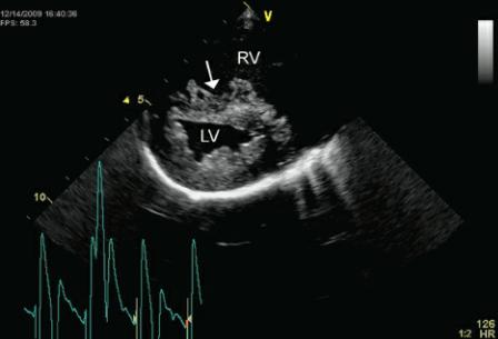
interventricular septum (arrow) on transverse left ventricular images. RV = right ventricle, LV = left ventricle.
References
1.Reef V. Advances in diagnostic ultrasonography. Vet Clin N Am: Eq Prac 1991;7:451–466.
2.Reef V. The use of diagnostic ultrasound in the horse. Ultras Quart 1991;9:1–33.
3.Reef V. Echocardiographic examination in the horse: the basics. Compendium 1990;12:1312–1320.
4.Reimer J. Cardiac evaluation of the horse: using ultrasonography. Vet Med 1993;88:748–755.
5.Miller M, Knauer K, Herring D. Echocardiography: principles of interpretation. Seminars Vet Med Surg (Sm Am) 1989;4:58–76.
6.Bonagura JD. Echocardiography. J AM Vet Med Assoc 1994;204:516–522.
7.Bonagura J, Herring D, Welker F. Echocardiography. Vet Clin N Am: Eq Prac 1985;1:311–333.
8.Bonagura J, O’Grady M, Herring D. Echocardiography. Vet Clin N Am: Sm Anim Prac 1985;15:1177–1194.
9.Bonagura J, Miller M. Veterinary echocardiography. Am J Cardiov Ultras & Allied Tech 1989;6:229–264.
10.Bonagura JD. M-mode echocardiography. Basic principles. Vet Clin North Am Small Anim Pract 1983; 13:299–319.
11.Miles K. Basic principles and clinical applications of diagnostic ultrasonography. Comp Sm Anim 1989;11:609–622.
12.Ettinger S, Lusk R. Echocardiographic techniques in the dog and cat. Proc 7th ACVIM 1989:229–
13.Kaplan P. Instrumentation, principles, and pitfalls of ultrasonography. Proc Vet Med 1991;3:457–
14.Lombard C, Evans M, Martin L, et al. Blood pressure, electrocardiogram and echocardiogram
measurements in the growing pony foal. Eq Vet J Suppl 1984;16:342–347.
15.Stewart J, Rose R, Barko A. Echocardiography in foals from birth to three months old. Eq Vet J Suppl 1984;16:332–341.
16.Long K, Bonagura J, Darke P. Standardized imaging technique for guided m-mode and Doppler echocardiography in the horse. Eq Vet J 1992;24:226–235.
17.Stadler P, Rewel A, Deegen E. M-mode echocardiography in dressage and show jumping horses of class “S” and in untrained horses. J Vet Med A 1993; 40:292–306.
18.Jacobs G, Knight D. M-mode echocardiographic measurements in nonanesthetized healthy cats: Effects of body weight, heart rate, and other variables. Am J Vet Res 1985;46:1705–1711.
19.Fox P, Bond B, Peterson M. Echocardiographic reference values in healthy cats sedated with ketamine hydrochloride. Am J Vet Res 1985;46:1479–1484.
20.DeMadron E, Bonagura J, Herring D. Two-dimensional echocardiography in the normal cat. Vet Rad 1985;26:149–158.
21.O’Grady M, Bonagura J, Powers J, et al. Quantitative cross-sectional echocardiography in the normal dog. Vet Rad Ultra 1986;27:34–49.
22.Mahony C, Rantanen N, DeMichael J, et al. Spontaneous echocardiographic contrast in the thoroughbred: high prevalence in racehorses and a characteristic abnormality in bleeders. Eq Vet J 1992;24:129–133.
23.Garcia-Fernandez M, Lopez-Sendon J, Coma-Canella I, et al. Echocardiographic detection of circulating blood in normal canine hearts. Am J Card 1985;56: 834–836.
24.Lang R, Bierig M, Devereux R, et al. Recommendations for chamber quantification. Eur J Echocardiogr 2006;7:79–108.
25.Sahn D, DeMaria A, Kisslo J, et al. Recommendations regarding quantitation in m-mode echocardiography: results of a survey of echocardiographic measurements. Circ 1978;58:1072–1083.
26.Troy B, Pombo J, Rackley C. Measurements of left ventricular wall thickness and mass by echocardiography. Circ 1972;45:602–611.
27.Wyatt H, Heng K, Weerbaum S, et al. Cross sectional echocardiography. Analysis of models for quantifying mass in the left ventricle in dogs. Circ 1983;60: 348–358.
28.Schiller N. Two-dimensional echocardiographic determination of left ventricular volume, systolic function, and mass. Summary and discussion of the 1989 recommendations of the American Society of Echocardiography. Circ 1991;84:I280–I287.
29.Schiller N, Skiôldebrand C, Schiller E, et al. Canine left ventricular mass estimation by twodimensional echocardiography. Circ 1983;68:210–216.
30.Lord P, Croft M. Accuracy of formulae for calculating left ventricular volumes of the equine heart. Eq Vet J Suppl 1990;9:53–56.
31.Bienvenu J, Drolet R. A quantitative study of cardiac mass in dogs. Can J Vet Res 1991;55:305–
32.Schiller N, Shah P, Crawford M, et al. Recommendations for quantification of the left ventricle by two-dimensional echocardiography. J Am Soc Echocard 1989;2:358–367.
33.Wyatt H, Heng M, Meerbaum S. Cross sectional echocardiography. I. Analysis of mathematical models for quantifying mass of the left ventricle in dogs. Circ 1979;60:1104–1113.
34.Rishniw M, Erb HN. Evaluation of four 2-dimensional echocardiographic methods of assessing left atrial size in dogs. Journal of Veterinary Internal Medicine 2000; 14:429–435.
35.Abbott JA, MacLean HN. Two-dimensional echocardiographic assessment of the feline left atrium. J Vet Intern Med 2006;20:111–119.
36.Voros K, Holmes J, Gibbs C. Anatomical validation of two-dimensional echocardiography in the horse. Eq Vet J 1990;22:392–397.
37.Voros K, Holmes J, Gibbs C. Measurement of cardiac dimensions with two-dimensional echocardiography in the living horse. Eq Vet J Suppl 1991;23:461–465.
38.O’Rourke R, Hanrath P, Henry W, et al. Report of the joint International Society and Federation of Cardiology/World Health Organization task force on recommendations for standardization of measurements from m-mode echocardiograms. Circ Suppl A 1984;69:854– 857.
39.Bonagura J. Echocardiography. JAVMA 1994;204:516–521.
40.Chetboul V, Tidholm A, Nicolle A, et al. Effects of animal position and number of repeated measurements on selected two-dimensional and M-mode echocardiographic variables in healthy dogs.
Journal of the American Veterinary Medical Association 2005;227:743–747.
41.Oyama M, Sisson D. Assessment of cardiac chamber size using anatomic m-mode. Vet Rad and Ultrasound 2005;46:331–336.
42.Lusk R, Ettinger S. Echocardiographic techniques in the dog and cat. J Am An Hosp Assoc 1990;26:473–488.
43.Mashiro I, Nelson R, Cohn J, et al. Ventricular dimensions measured noninvasively by echocardiography in the awake dog. J App Physiol 1976;41:953–959.
44.Jacobs G, Mahjoob K. Multiple regression analysis, using body size and cardiac cycle length, in predicting echocardiographic variables in dogs. Am J Vet Res 1988;49:1290–1294.
45.Jacobs G, Mahjoob K. Influence of alterations in heart rate on echocardiographic measurements in the dog. Am J Vet Res 1988;49:548–552.
46.Lombard C. Normal values of the canine m-mode echocardiogram. Am J Vet Res 1984;45:2015– 2018.
47.Sisson D, Schaeffer D. Changes in linear dimensions of the heart, relative to body weight, as measured by m-mode echocardiography in growing dogs. Am J Vet Res 1991;52:1591–1596.
48.Snyder P, Sato T, Atkins C. A comparison of echocardiographic indices of the nonracing, healthy greyhound to reference values from other breeds. Vet Rad & Ultras 1995;36:387–392.
49.Page A, Edmunds G, Atwell R. Echocardiographic values in the greyhound. Aust Vet J 1993;70:361–364.
50.Boon J, Wingfield W, Miller C. Echocardiographic indices in the normal dog. Vet Rad Ultra 1983;24: 214–221.
51.Bayón A, Fernández del Palacio J, Montes A, et al. M-mode echocardiography study in growing Spanish mastiffs. J Sm An Prac 1994;35:473–479.
52.Crippa L, Ferro E, Melloni E, et al. Echocardiographic parameters and indices in the normal Beagle dog. Lab Anim 1992;26:190–195.
53.Gooding J, Robinson W, Mews G. Echocardiographic assessment of left ventricular dimensions in clinically normal English Cocker Spaniels. Am J Vet Res 1986;47:296–300.
54.Morrison S, Moise N, Scarlett J, et al. Effect of breed and body weight on echocardiographic values in four breeds of dogs of differing somatype. J Vet Int Med 1992;6:220–224.
55.Allen D. Echocardiographic study of the anesthetized cat. Can J Comp Med 1982;46:115–122.
56.Allen D, Downey R. Echocardiographic assessment of cats anesthetized with xylazine-sodium pentobarbital. Can J Comp Med 1983;47:281–283.
57.Jacobs G, Knight D. Change in m-mode echocardiographic values in cats given ketamine. Am J Vet Res 1985;46:1712–1713.
58.Moise N, Dietze A. Echocardiographic, electrocardiographic, and radiographic detection of cardiomegaly in hyperthyroid cats. Am J Vet Res 1986;47:1487–1494.
59.Moise N, Horne W, Flanders J, et al. Repeatability of the M-mode echocardiogram and the effects of acute changes in heart rate, cardiac contractility, and preload in healthy cats sedated with ketamine hydrochloride and acepromazine. Cornell Vet 1986;76:241–258.
60.Moise N, Dietze A, Mezza L, et al. Echocardiography, electrocardiography, and radiography of cats with dilation cardiomyopathy, hypertrophic cardiomyopathy, and hyperthyroidism. Am J Vet Res 1986;47:1476–1486.
61.Pipers F, Reef V, Hamlin R. Echocardiography in the domestic cat. Am J Vet Res 1979;40:882–
62.Pipers F, Hamlin R. Clinical use of echocardiography in the domestic cat. JAVMA 1980;176:57–
63.Sisson DD, Knight DH, Helinski C, et al. Plasma taurine concentrations and M-mode echocardiographic measures in healthy cats and in cats with dilated cardiomyopathy. J Vet Intern Med 1991;5:232–238.
64.Soderberg S, Boon J, Wingfield W, et al. M-mode echocardiography as a diagnostic aid for feline cardiomyopathy. Vet Rad Ultra 1983;24:66–73.
65.Lombard C, Evans M, Martin L, et al. Blood Pressure, electrocardiogram and echocardiogram measurements in the growing pony foal. Equine Vet J Suppl 1984;16: 342–347.
66.Lescure F, Tamzali Y. Referring values in echocardiography TM in sport-horse. Revue Med Vet 1984;135: 405–418.
67.Bertone J, Paull K, Wingfield W, et al. M-mode echocardiography of endurance horses in the recovery phase of long-distance competition. Am J Vet Res 1987; 48:1708–1712.
68.O’Callaghan M. Comparison of echocardiographic and autopsy measurements of cardiac dimensions in the horse. Eq Vet J Suppl 1985;17:361–368.
69.Paull K, Wingfield W, Bertone J, et al. Echocardiographic changes with endurance training. In: Gillespie J, Robinson N, eds. Equine Excercise Physiology 2. Davis, Calif: ICEEP Publications, 1987;34–40.
70.Pipers F, Hamlin R. Echocardiography in the horse. JAVMA 1977;170:815–819.
71.Moses B, Ross J. M-mode echocardiographic values in sheep. Am J Vet Res 1987;48:1313–1318.
72.Pipers F, Muir W, Hamlin R. Echocardiography in swine. Am J Vet Res 1978;39:707–710.
73.Gwathmey J, Nakao S, Come P, et al. Echocardiographic assessment of cardiac chamber size and functional performance in swine. Am J Vet Res 1989;50:192–197.
74.Boon JA, Knight AP, Moore DH. Llama cardiology. Vet Clin North Am Food Anim Pract
1994;10:353–370.
75.Amory H, Kafidi N, Lekeux P. Echocardiographic evaluation of cardiac morphologic and functional variables in double-muscled calves. Am J Vet Res 1992;53:1540–1547.
76.Amory H, Jakovljevic S, Lekeux P. Quantitative M-mode and two-dimensional echocardiography in calves. Vet Rec 1991;128:25–31.
77.Amory H, Lekeux P. Effects of growth on functional and morphological echocardiographic variables in Friesian calves. Vet Rec 1991;128:349–354.
78.Pipers F, Reef V, Hamlin R, et al. Echocardiography in the bovine animal. Bov Prac 1978;13:114–
79.Gaasch W. Left ventricular radius to wall thickness ratio. Am J Card 1979;43:1189–1194.
80.Grossman W, Jones D, McLaurin L. Wall stress and patterns of ventricular hypertrophy in the human left ventricle. J Clin Invest 1975;56:56–64.
81.Titcomb C. LVH: Consequences associated with cardiac remodeling. J Insur Med 2004;36:42–46.
82.Quinones M, Mokotoff D, Nouri S, et al. Noninvasive quantification of left ventricular wall stress. Validation of method and application to assessment of chronic pressure overload. Am J Card 1980;45:782–790.
83.Paul JJ, Tani LY, Williams RV, et al. Relation of the discrete subaortic stenosis position to mitral valve function. Am J Cardiol 2002;90:1414–1416.
84.Kirberger R. Mitral valve E point to ventricular septal separation in the dog. Tydskr S Afr Vet Ver 1991;62: 163–166.
85.Child J, Krivokapich J, Perloff J. Effect of left ventricular size on mitral E point to ventricular septal separation in assessment of cardiac performance. Am Heart J 1981;101:797–805.
86.Ginzton L, Kulick D. Mitral valve E-point septal separation as an indicator of ejection fraction in patients with reversed septal motion. Chest 1985;88:429–431.
87.Brown O, Harrison D, Popp R. An improved method for detection of left atrial enlargement. Circ 1974;50:58–64.
88.Kienle R. Echocardiography In: Kittleson M,Kienle R, eds. Small Animal Cardiovascular Medicine. St. Louis: Mosby, 1998;95–117.
89.Brown D, Rush J, MacGregor J, et al. M-mode echocardiographic ratio indices in normal dogs, cats, and horses: A novel quantitative method. J Vet Intern Med 2003;17:653–662.
90.Bonagura J, Darke P, Long K, et al. Doppler-echocardiographic estimation of heart function: comparison with invasive measurement in closed-chest dogs. Proc 8th ACVIM Forum 1990:863–866.
91.Darke P. An evaluation of transducer sites for measurement of aortic and pulmonary flows by Doppler echocardiography. Proc 9th ACVIM 1991:703–705.
92.Darke P. Two-dimensional imaging for Doppler echocardiography in dogs. Proc 8th ACVIM 1990:261– 268.
93.Darke P, Bonagura J, Miller M. Transducer orientation for Doppler echocardiography in dogs. J Sm An Prac 1993;34:2–8.
94.Kirberger R, Bland-van den Berg P, Darazs B. Doppler echocardiography in the normal dog: Part I, Velocity findings and flow patterns. Vet Rad Ultra 1992;33: 370–379.
95.Kirberger R, Bland-van den Berg P, Grimbeek R. Doppler echocardiography in the normal dog:
Part II, Factors influencing blood flow velocities and a comparison between left and right heart blood flow. Vet Rad Ultra 1992;33:380–386.
96.Long K. Doppler echocardiography in the horse. Eq Vet Ed 1990;2:15–17.
97.Gaber C. Doppler Echocardiography. Prob Vet Med 1991;3:479–499.
98.Darke P. Doppler echocardiography. J Sm Anim Prac 1992;33:104–112.
99.Hatle L, Angelsen B. Doppler Ultrasound in Cardiology. Physical Principles and Clinical Applications. 2nd ed. Philadelphia: Lea and Febiger, 1985.
100.Brown D, Knight D, King R. Use of pulsed-wave Doppler echocardiography to determine aortic and pulmonary velocity and flow variables in clinically normal dogs. Am J Vet Res 1991;52:543–550.
101.Yuill C, O’Grady M. Doppler-derived velocity of blood flow across the cardiac valves in the normal dog. Can J Vet Res 1991;55:185–192.
102.Reef V, Lalezari K, De Boo J, et al. Pulsed-wave Doppler evaluation of intracardiac blood flow in
30clinically normal Standardbred horses. Am J Vet Res 1989;50:75–83.
103.Yamamoto K, Masuyama T, Tanouchi J, et al. Effects of heart rate on left ventricular filling dynamics: assessment from simultaneous recordings of pulsed Doppler transmitral flow velocity pattern and haemodynamic variables. Card Res 1993;27:935–941.
104.Gaber C. Normal pulsed wave Doppler flow velocities in adult dogs. Proc 5th ACVIM 1987:923.
105.Kirberger R. Pulsed wave Doppler echocardiographic evaluation of intracardiac blood flow in normal sheep. Res Vet Sci 1993;55:189–194.
106.Gaber C. Normal pulsed Doppler flow velocities in adult dogs. Proc 5th ACVIM 1987:923.
107.Blissitt K, Bonagura J. Pulsed wave Doppler echocardiography in normal horses. Eq Vet J Suppl 1995;19: 38–46.
108.Stadler P, Weinberger T, Deegen E. Pulsed Doppler echocardiography in healthy warm blooded horses. J Vet Med A 1993;40:757–778.
109.Atkins C, Snyder P. Systolic time intervals and their derivatives for evaluation of cardiac function. J Vet Int Med 1992;6:55–63.
110.Lewis R, Rittgers S, Forester W, et al. A critical review of the systolic time intervals. Circ 1977; 56:146–158.
111.Santilli RA, Bussadori C. Doppler echocardiographic study of left ventricular diastole in nonanaesthetized healthy cats. Vet J 1998;156:203–215.
112.Lester SJ, Tajik AJ, Nishimura RA, et al. Unlocking the mysteries of diastolic function: deciphering the Rosetta Stone 10 years later. J Am Coll Cardiol 2008;51: 679–689.
113.Schober KE, Fuentes VL. Effects of age, body weight, and heart rate on transmitral and pulmonary venous flow in clinically normal dogs. American Journal of Veterinary Research 2001;62:1447–1454.
114.Fuentes VL. Diastolic function—is this the key to successful management of many feline cardiomyopathies? J Feline Med Surg 2003;5:51–56.
115.Thomas J, Weyman A. Echocardiographic Doppler evaluation of left ventricular diastolic function. Physics and physiology. Circulation 1991;84:977–990.
116.Schober KE, Fuentes VL, Bonagura JD. Comparison between invasive hemodynamic measurements and noninvasive assessment of left ventricular diastolic function by use of Doppler
echocardiography in healthy anesthetized cats. American Journal of Veterinary Research 2003;64:93– 103.
117.Nishamura R, Abel M, Hatle L, et al. Assessment of diastolic function of the heart: background and current applications of Doppler echocardiography. Part II: clinical studies. Mayo Clin Proc 1989;64:181–204.
118.Nishamura R, Housmans P, Hatle L, et al. Assessment of diastolic function of the heart: background and current applications of Doppler echocardiography. Part I. Physiologic and pathophysiologic features. Mayo Clin Proc 1989;64:71–81.
119.Disatian S, Bright JM, Boon J. Association of age and heart rate with pulsed-wave Doppler measurements in healthy, nonsedated cats. J Vet Intern Med 2008;22: 351–356.
120.Nishimura RA, Tajik AJ. Evaluation of diastolic filling of left ventricle in health and disease: Doppler echocardiography is the clinician’s Rosetta Stone. J Am Coll Cardiol 1997;30:8–18.
121.Wilansky S. Two-dimensional and Doppler echocardiography for the assessment of congestive heart failure. Texas Heart Institute Journal 1998;25:260–264.
122.Thomas J, Flachskampf F, Chen C, et al. Isovolumic relaxation time varies predictably with its time constant and aortic and left atrial pressures: Implications for the noninvasive evaluation of ventricular relaxation. Am Heart J 1992;124:1305–1313.
123.Plotnick G. Changes in diastolic function—Difficult to measure, harder to interpret. Am Heart J 1989;118: 637–641.
124.Schober KE, Maerz I. Doppler echocardiographic assessment of left atrial appendage flow velocities in normal cats. Journal of Veterinary Cardiology 2005;7: 15–25.
125.Schober K, Maerz I. Assessment of left atrial appendage flow velocity and its relation to spontaneous echocardiographic contrast in 89 cats with myocardial disease. Journal of Veterinary Internal Medicine 2006;20:120–130.
126.Chetboul V. Tissue Doppler imaging: a promising technique for quantifying regional myocardial function. J Vet Cardiol 2002;4:7.
127.Chetboul V, Sampedrano CC, Tissier R, et al. Quantitative assessment of velocities of the annulus of the left atrioventricular valve and left ventricular free wall in healthy cats by use of twodimensional color tissue Doppler imaging. Am J Vet Res 2006;67:250–258.
128.Chetboul V, Sampedrano CC, Tissier R, et al. Reference range values of regional left ventricular myocardial velocities and time intervals assessed by tissue Doppler imaging in young nonsedated Maine Coon cats. American Journal of Veterinary Research 2005;66:1936–1942.
129.Chetboul V, Athanassiadis N, Carlos C, et al. Quantification, repeatability, and reproducibility of feline radial and longitudinal left ventricular velocities by tissue Doppler imaging. American Journal of Veterinary Research 2004;65:566–572.
130.Simpson KE, Devine BC, Gunn-Moore DA, et al. Assessment of the repeatability of feline echocardiography using conventional echocardiography and spectral pulse-wave Doppler tissue imaging techniques. Vet Radiol Ultrasound 2007;48:58–68.
131.Schwarzwald CC, Schober KE, Bonagura JD. Methods and reliability of echocardiographic assessment of left atrial size and mechanical function in horses. Am J Vet Res 2007;68:735–747.
132.Sepulveda M, Perkins J, Bowen I, et al. Demonstration of regional differences in equine ventricular myocardial velocity in normal 2 year old Thoroughbreds with tissue Doppler imaging. Eq
Vet J 2005;37:222–226.
133.Chetboul V, Sampedrano CC, Gouni V, et al. Quantitative assessment of regional right ventricular myocardial velocities in awake dogs by Doppler tissue imaging: repeatability, reproducibility, effect of body weight and breed, and comparison with left ventricular myocardial velocities. J Vet Intern Med 2005;19:837–844.
134.Disatian S, Bright J, Boon J. The effects of age and heart rate on tricuspid annular motion velocities in healthy nonsedated cats. J Vet Int Med 2007;21:731–736.
135.Chetboul V, Sampedrano CC, Concordet D, et al. Use of quantitative two-dimensional color tissue Doppler imaging for assessment of left ventricular radial and longitudinal myocardial velocities in dogs. Am J Vet Res 2005;66:953–961.
136.Koffas H, Dukes-McEwan J, Corcoran BM, et al. Peak mean myocardial velocities and velocity gradients measured by color M-mode tissue Doppler imaging in healthy cats. J Vet Intern Med 2003;17:510–524.
137.Wess G, Killich M, Wagner T, et al. Comparison of two methods to measure tissue Doppler velocities. ACVIM 2006;773.
138.Chetboul V, Athanassiadis N, Carlos C, et al. Quantification, repeatability, and reproducibility of feline radial and longitudinal left ventricular velocities by tissue Doppler imaging. Am J Vet Res 2004;65: 566–572.
139.Killich M, Hartmann K, Wess G. Influence of age, weight and breed on longitudinal systolic tissue Doppler modalities. ECVIM 2007;1441.
140.Hori Y, Ukai Y, Hoshi F, et al. Volume loading-related changes in tissue Doppler images derived from the tricuspid valve annulus in dogs. Am J Vet Res 2008;69: 33–38.
141.Choong C, Abascal V, Weyman J, et al. Prevalence of valvular regurgitation by Doppler echocardiography in patients with structurally normal hearts by two dimensional echocardiography. Am Heart J 1989;117:636–642.
142.Sahn D, Maciel B. Physiological valvular regurgitation. Doppler echocardiography and the potential for iatrogenic heart disease. Circ 1989;78:1075–1077.
143.Blissitt K, Bonagura J. Colour flow Doppler echocardiography in horses with cardiac murmurs. Eq Vet J Suppl 1995;19:82–85.
144.Marr C, Reef V. Physiological valvular regurgitation in clinically normal young racehorses: prevalence and two dimensional colour flow Doppler echocardiographic characteristics. Eq Vet J Suppl 1995;19:56–62.
145.Nakayama T, Wakao Y, Takiguchi S, et al. Prevalence of valvular regurgitation in normal beagle dogs detected by color Doppler echocardiography. J Vet Med Sci 1994;56:973–975.
146.Kostucki W, Vandenbossche J, Friart A, et al. Pulsed Doppler regurgitant flow patterns of normal valves. Am J Card 1986;58:309–313.
147.Yock P, Naasz C, Schnittger I, et al. Doppler tricuspid and pulmonic regurgitation in normals: is it real? Circ 1984;70(suppl II):40.
148.Blissitt K, Bonagura J. Colour flow Doppler echocardiography in normal horses. Eq Vet J Suppl 1995;19: 47–55.
149.Pollak S, McMillan S, Knopff W, et al. Cardiac evaluation of women distance runners by
echocardiographic color flow mapping. J Am Col Cardiol 1988;11:89–93.
150.Helmcke F, Nanda N, Hsiung M, et al. Color Doppler assessment of mitral regurgitation with orthogonal planes. Circ Res 1987;75:175–183.
151.Cooper J, Nanda N, Philpot E, et al. Evaluation of valvular regurgitation by color Doppler. J Am Soc Echocardiogr 1989;2:56–66.
152.Braunwald E. Pathophysiology of heart failure In: Braunwald E, ed. Heart Disease: A Textbook of Cardiovascular Medicine. Philadelphia: WB Saunders Co, 1980;453–471.
153.Schlant R, Sonnenblick E. Pathophysiology of heart failure. In: Hurst J, Schlant R, Rackley C, et al., eds. The Heart. 7 ed. New York: McGraw Hill Book Co, 1990; 387–418.
154.Hirota Y. A clinical study of left ventricular relaxation. Circ 1980;62:756–763.
155.Atkins C, Curtis M, McGuirk S, et al. The use of m-mode echocardiography in determining cardiac output in dogs with normal, low, and high output states: comparison to thermodilution method. Vet Rad Ultras 1992;33:297–304.
156.Federman M, Hess O. Differentiation between systolic and diastolic dysfunction. Eur Heart J Suppl D 1994; 15:2–6.
157.Kittleson M. Left ventricular function and failure—part I. Comp Sm Anim 1994;16:287–308.
158.Kittleson M. Left ventricular function and failure—part II. Comp Sm Anim 1994;16:1001–1017.
159.Aurigemma G, Douglas P, Gaasch W. Quantitative evaluation of left ventricular structure, wall stress, and systolic function. In: Otto C, ed. The practice of Clinical Echocardiography. 2nd ed. Philadelphia: WB Saunders Company, 2002;65–87.
160.Mebazaa A, Karpati P, Renaud E, et al. Acute right ventricular failure—from pathophysiology to new treatments. Inten Care Med 2004;30:185–196.
161.Redington A, Rigby M. Changes in the pressure volume relation of the right ventricle when its loading conditions are modified. Br Heart J 1990;63:45–49.
162.Hess B, Asher C. Time to move to the right—the study of right ventricular systolic performance: too long neglected. Clin Cardiol 2005;28:8–12.
163.Teicholz L, Kreulen T, Herman M, et al. Problems in echocardiographic volume determinations: echocardiographic—angiographic correlations in the presence or absence of asynergy. Am J Card 1976; 37:7–11.
164.Kronik G, Slany J, Mösslacher H. Comparative value of eight m-mode echocardiographic formulas for determining left ventricular stroke volume. A correlative study with thermodilution and left ventricular single plane cineangiography. Circ 1979;60:1308–1316.
165.Uehara Y, Koga M, Takahashi M. Determination of cardiac output by echocardiography. J Vet Med Sci 1995;57:401–407.
166.Sisson D, Daniel G, Twardock A. Comparison of left ventricular ejection fractions determined in healthy anesthetized dogs by echocardiography and gated equilibrium radionuclide ventriculography. Am J Vet Res 1989;50:1840–1847.
167.Serres F, Chetboul V, Tissier R, et al. Comparison of 3 ultrasound methods for quantifying left ventricular systolic function: Correlation with disease severity and prognostic value in dogs with mitral valve disease. J Vet Int Med 2008;22.
168.Dyson D, Allen D, McDonell W. Comparison of three methods for cardiac output determination
in cats. Am J Vet Res 1985;46:2546–2552.
169.Kittleson M, Eyster G, Knowlen G, et al. Myocardial function in small dogs with chronic mitral regurgitation and severe congestive heart failure. JAVMA 1985; 184:1253–1256.
170.Jardin F, Viellard-Baron A. Monitoring of right sided function. Curr Opin Crit Care 2005;11:271–279.
171.Guarracino F, Cariello C, Doroni D, et al. Right ventricular failure: physiology and assessment.
Minerva Anesthiol 2005;71:307–312.
172.Pipers F, Andrysco R, Hamlin R. A totally noninvasive method for obtaining systolic time intervals in the dog. AM J Vet Res 1978;39:1822–1826.
173.Hassan S, Turner P. Systolic time intervals: A review of the method in the non-invasive investigation of cardiac function in health, disease and clinical pharmacology. Postgrad Med J 1983; 59:423–434.
174.Weissler A. Current concepts in cardiology; systolic time intervals. N Eng J Med 1977;296:321–
175.Emilsson K, Alam M, Wandt B. The relation between mitral annulus motion and ejection fraction: a nonlinear function. J Am Soc Echocardiogr 2000;13:896–901.
176.Schober KE, Fuentes VL. Mitral annulus motion as determined by m-mode echocardiography in normal dogs and dogs with cardiac disease. Veterinary Radiology & Ultrasound 2001;42:52–61.
177.Ghio S, Recusani F, Klersy C, et al. Prognostic usefulness of the tricuspid annular plane systolic excursion in patients with congestive heart failure secondary to idiopathic or ischemic dilated cardiomyopathy. Am J Card 2000;85:837–842.
178.Dini F, Conti U, Fontanive P, et al. Right ventricular dysfunction is a major predictor of outcome in patients with moderate to severe mitral regurgitation and left ventricular dysfunction. Am Heart J 2007;154:172–179.
179.Allen D, Nymeyer D. A preliminary investigation on the use of thermodilution and echocardiography as an assessment of cardiac function in the cat. Can J Comp Med 1983;47:112–117.
180.McGowan J, Cleland J. Reliability of reporting left ventricular systolic function by echocardiography: a systematic review of 3 methods. Am Heart J 2003;146: 388–397.
181.Wyatt H, Heng M, Meerbaum S, et al. Cross sectional echocardiography II. Analysis of mathematical models for quantifying volume of the formalin fixed left ventricle. Circ 1980;61:1119– 1125.
182.Vörös K, Holmes J, Gibbs C. Left ventricular volume determination in the horse by twodimensional echocardiography: an in vitro study. Eq Vet J 1990;22: 398–401.
183.Zogbbi W, Quinones M. Determination of cardiac output by Doppler echocardiography: a critical appraisal. Herz 1986;11:258–268.
184.Huntsman L, Stewart D, Barnes S, et al. Noninvasive Doppler determination of cardiac output in man: clinical validation. Circ 1983;67:593–602.
185.Fisher D, Sahn D, Friedman M, et al. The mitral valve orifice method for noninvasive twodimensional echo Doppler determination of cardiac output. Circ 1983; 67:872–877.
186.Nishimura R, Tajik A. Quantitative hemodynamics by Doppler echocardiography: a noninvasive alternative to cardiac catheterization. Prog Cardiov Dis 1994;36: 309–342.
187.Quiñones MA, Otto CM, Stoddard M, et al. Recommendations for quantification of Doppler echocardiography: a report from the Doppler Quantification Task Force of the Nomenclature and Standards Committee of the American Society of Echocardiography. J Am Soc Echocardiogr 2002;15:167–184.
188.Labovitz A, Buckingham T, Habermehl K, et al. The effects of sampling site on the two dimensional echo-Doppler determination of cardiac output. Am Heart J 1985;109:327–332.
189.Stewart W, Jiang L, Mick R, et al. Variable effects of change in flow rate through the aortic, pulmonary and mitral valves on valve area and flow velocity: impact on quantitative Doppler flow calculations. J Am Col Cardiol 1985;6:653–662.
190.Valdes-Cruz L, Horowitz S, Mesel E, et al. A pulsed Doppler method for calculation of pulmonary and systemic flow: accuracy in a canine model with ventricular septal defect. Circ 1983;68:597–602.
191.Ascah K, Stewart W, Gillam L, et al. Calculation of transmitral flow by Doppler echocardiography: a comparison of methods in a canine model. Am Heart J 1989;117:402–411.
192.Bennett E, Barclay S, Davis A, et al. Ascending aortic blood velocity and acceleration using Doppler ultrasound in the assessment of left ventricular function. Cardiovasc Res 1984;18:632–638.
193.Sabbath H, Khaja F, Brymer J, et al. Noninvasive evaluation of left ventricular performance based peak aortic blood acceleration measured with a continuous wave Doppler velocity meter. Circ 1986;74:323–329.
194.Sabbath H, Gheorghiade M, Smith S, et al. Serial evaluation of left ventricular function in congestive heart failure by measurement of peak aortic blood acceleration. Am J Cardiol 1988;57:367–370.
195.Dujardin K, Tei C, Yeo T, et al. Prognostic value of a Doppler index combining systolic and diastolic performance in idiopathic-dilated cardiomyopathy. Am J Card 1998;82:1071–1076.
196.Teshima K, Asano K, Sasaki Y, et al. Assessment of left ventricular function using pulsed tissue Doppler imaging in healthy dogs and dogs with spontaneous mitral regurgitation. J Vet Med Sci 2005;67:1207–1215.
197.Teshima K, Asano K, Iwanaga K, et al. Evaluation of right ventricular tei index (index of myocardial performance) in healthy dogs and dogs with tricuspid regurgitation. J Vet Med Sci 2006;68:1307–1313.
198.Lee B, Dukes-McEwan J, French A, et al. Evaluation of a novel Doppler index of combined systolic and diastolic myocardial performance in Newfoundland dogs with familial prevalence of dilated cardiomyopathy. Vet Rad and Ultrasound 2002;43:154–165.
199.Teshima K, Asano K, Iwanaga K, et al. Evaluation of left ventricular tei index (index of myocardial performance) in healthy dogs and dogs with mitral regurgitation. J Vet Med Sci 2007;69:117–123.
200.Hori Y, Kunihiro S, Hoshi F, et al. Comparison of the myocardial performance index derived by use of pulsed Doppler echocardiography and tissue Doppler imaging in dogs with volume overload.
American Journal of Veterinary Research 2007;68:1177–1182.
201.Hori Y, Uechi M, Indou A, et al. Changes in the myocardial performance index during dobutamine administration in anesthetized cats. American Journal of Veterinary Research 2007;68:385–388.
202.Hori Y, Kunihiro S, Hoshi F, et al. Comparison of the myocardial performance index derived by use of pulsed Doppler echocardiography and tissue Doppler imaging in dogs with volume overload. Am J Vet Res 2007;68: 1177–1182.
203.Hori Y, Uechi M, Indou A. Effects of changes in loading conditions and heart rate on the myocardial performance index in cats. Am J Vet Res 2007;68:1183– 1187.
204.Baumwart R, Meuers K, Bonagura J. Tei index of myocardial performance applied to the right ventricle in dogs. J Vet Int Med 2005;19.
205.Cheung M, Smallhorn J, Redington A, et al. The effects of changes in loading conditions and modulation of inotropic state on the myocardial performance index: comparison with conductance catheter measurements. Eur Heart J 2004;25:2185–2186.
206.Ishii M, Eto G, Tei C, et al. Quantitation of the global right ventricular function in children with normal heart and congenital heart disease: A right ventricular myocardial performance index. Pediatr Cardiol 2000;21: 416–421.
207.Chetboul V, Carlos C, Blot S, et al. Tissue Doppler assessment of diastolic and systolic alterations of radial and longitudinal left ventricular motions in Golden Retrievers during the preclinical phase of cardiomyopathy associated with muscular dystrophy. Am J Vet Res 2004;65:1335– 1341.
208.Chetboul V, Gouni V, Sampedrano CC, et al. Assessment of regional systolic and diastolic myocardial function using tissue Doppler and strain imaging in dogs with dilated cardiomyopathy. J Vet Intern Med 2007;21: 719–730.
209.Chetboul V, Carlos Sampedrano C, Testault I, et al. Use of tissue Doppler imaging to confirm the diagnosis of dilated cardiomyopathy in a dog with equivocal echocardiographic findings. Journal of the American Veterinary Medical Association 2004;225:1877–1880.
210.Chetboul V, Escriou C, Tessier D, et al. Tissue Doppler imaging detects early asymptomatic myocardial abnormalities in a dog model of Duchenne’s cardiomyopathy. Eur Heart J 2004;25:1934– 1939.
211.O’Sullivan M, O’Grady M, Minors S. Assessment of diastolic function by Doppler echocardiography in normal Doberman Pinschers and Doberman Pinschers with dilated cardiomyopathy. Journal of Veterinary Internal Medicine 2007;21:81–91.
212.Tabata T, Cardon L, Armstrong G, et al. An evaluation of the use of new Doppler methods for detecting longitudinal function abnormalities in a pacing-induced heart failure model. J Am Soc Echocardiogr 2003;16: 424–431.
213.Yu CM, Sanderson JE, Marwick TH, et al. Tissue Doppler imaging a new prognosticator for cardiovascular diseases. J Am Coll Cardiol 2007;49:1903–1914.
214.Agricola E, Galderisi M, Oppizzi m, et al. Pulsed tissue Doppler imaging detects early myocardial dysfunction in asymptomatic patients with severe mitral regurgitation. Heart 2004;90:406–410.
215.Hori Y, Sato S, Hoshi F, et al. Assessment of longitudinal tissue Doppler imaging of the left ventricular septum and free wall as an indicator of left ventricular systolic function in dogs. Am J Vet Res 2007;68: 1051–1057.
216.Chetboul V, Carlos C, Blot S, et al. Tissue Doppler assessment of diastolic and systolic alterations of radial and longitudinal left ventricular motions in Golden Retrievers during the
preclinical phase of cardiomyopathy associated with muscular dystrophy. Am J Vet Res 2004;65:1335– 1341.
217.Koffas H, Dukes-McEwan J, Corcoran M, et al. Pulsed tissue Doppler imaging in normal cats and cats with hypertrophic cardiomyopathy. Journal of Veterinary Internal Medicine 2006;20:65–77.
218.Chetboul V, Blot S, Sampedrano C, et al. Tissue Doppler imaging for detection of radial and longitudinal myocardial dysfunction in a family of cats affected by dystrophin-deficient hypertrophic muscular dystrophy. J Vet Int Med 2006;20:640–647.
219.Meluzín J, Spinarová L, Bakala J, et al. Pulsed Doppler tissue imaging of the velocity of tricuspid annular systolic motion; a new, rapid, and non-invasive method of evaluating right ventricular systolic function. Eur Heart J 2001;22:340–348.
220.Ho C, Solomon S. A clinician’s guide to tissue Doppler imaging. Circ 2006;113:e396–e398.
221.Saxena N, Rajagopalan N, Edelman K. Tricuspid annular systolic velocity: A useful measurement in determining right ventricular systolic function regardless of pulmonary artery pressures.
Echocardiography 2006;23:750–755.
222.Serres F, Chetboul V, Gouni V, et al. Diagnostic value of echo-Doppler and tissue Doppler imaging in dogs with pulmonary arterial hypertension. J Vet Intern Med 2007;21:1280–1289.
223.DeMaria A, Wisenbaugh T, Smith M, et al. Doppler Echocardiographic evaluation of diastolic function. Circ Suppl I 1991;84:288–295.
224.Dougherty A, Naccarelli G, Gray E, et al. Congestive heart failure with normal systolic function. Am J Card 1984;54:778–782.
225.Soufer R, Wohlgelernter D, Vita N, et al. Intact systolic left ventricular function in clinical congestive heart failure. Am J Card 1984;53:567–571.
226.Brutsaert D, Rademakers F, Sys S, et al. Analysis of relaxation in the evaluation of ventricular function of the heart. Prog Cardiovasc Dis 1985;28:143–163.
227.Yellin E, Nikolic S, Frater R. Left ventricular filling dynamics and diastolic function. Prog Cardiovasc Dis 1990;32:242–271.
228.Kamp O. Advanced systolic and diastolic function: beyond the E and A wave. Sem Cardiothoracic and Vascular Anethesia 2006;10:63–65.
229.Guarracino F, Lapolla F, Danella A, et al. Reduced compliance of left ventricle. Minerva Anestesiol 2004;70:225–228.
230.Nishimura R, Appleton C, Redfield M, et al. Noninvasive Doppler echocardiographic evaluation of left ventricular filling pressures in patients with cardiomyopathies: a simultaneous Doppler echocardiographic and cardiac catheterization study. J Am Coll Cardiol 1996;28:1226– 1233.
231.Borgarelli M, Santilli RA, Chiavegato D, et al. Prognostic indicators for dogs with dilated cardiomyopathy. J Vet Intern Med 2006;20:104–110.
232.MacDonald A, Kittleson M, Garcia-Nolen T, et al. Tissue Doppler imaging and gradient echo cardiac magnetic resonance imaging in normal cats and cats with hypertrophic cardiomyopathy. J Vet Int Med 2006;20:627–634.
233.Wang M, Yip GW, Wang AY, et al. Peak early diastolic mitral annulus velocity by tissue Doppler imaging adds independent and incremental prognostic value. J Am Coll Cardiol 2003;41:820–
234.Gavaghan B, Kittleson M, Fisher K, et al. Quantification of left ventricular diastolic wall motion by Doppler tissue imaging in healthy cats and cats with cardiomyopathy. Am J Vet Res 1999;60:1478– 1486.
235.Hasegawa H, Little W, Ohno M, et al. Diastolic annular velocity during the development of heart failure. J Am Col Cardiol 2003;41:1590–1597.
236.Ohno M, Cheng C, Little W. Mechanism of altered patterns of left ventricular filling during the development of congestive heart failure. Circ 1994;89:2241–2250.
237.Capomolla S, Pinna G, Febo O, et al. Echo Doppler mitral flow monitoring: an operative tool to evaluate tolerance to and effectiveness of beta adrenergic blocking agent therapy in patients with chronic heart failure. J Am Col Cardiol 2001;38:1675–1684.
238.Callahan M, Tajik A, Su-Fan Q, et al. Validation of instantaneous pressure gradients measured by continuous wave Doppler in experimentally induced aortic stenosis. Am J Card 1995;56:989–993.
239.Tou SP, Adin DB, Estrada AH. Echocardiographic estimation of systemic systolic blood pressure in dogs with mild mitral regurgitation. J Vet Intern Med 2006;20: 1127–1131.
240.Uehara Y. An attempt to estimate the pulmonary artery pressure in dogs by means of pulsed Doppler echocardiography. J Vet Med Sci 1993;55:307–312.
241.Teague S, Heinsimer J, Anderson J, et al. Quantification of aortic regurgitation utilizing continuous wave Doppler ultrasound. J AM Coll Card 1986;8:592–599.
242.Fox PR, Miller MW, Liu SK. Clinical, echocardiographic, and Doppler imaging characteristics of mitral valve stenosis in two dogs. J Am Vet Med Assoc 1992;201: 1575–1579.
243.Lehmkuhl LB, Ware WA, Bonagura JD. Mitral stenosis in 15 dogs. J Vet Intern Med 1994;8:2–
244.Stamoulis M, Fox P. Mitral valve stenosis in three cats. J Sm Anim Prac 1993;34:452–456.
245.Oyama MA, Weidman JA, Cole SG. Calculation of pressure half-time. Journal of Veterinary Cardiology 2008; 10:57–60.
246.Lewis B, Hasin Y, Pasternak R, et al. Echocardiographic aortic root motion in ventricular volume overload and the effect of mitral incompetence. Eur J Card 1979;10: 375–384.
247.Gilbert B, Pollick C, Adelman A, et al. Hypertrophic cardiomyopathy: subclassification by m- mode echocardiography. Am J Card 1980;45:861–872.
248.Krajcer Z, Orzan F, Pechacek L, et al. Early systolic closure of the aortic valve in patients with hypertrophic subaortic stenosis and discrete subaortic stenosis. Am J Cardiol 1978;41:823–829.
249.Gardin J, Tommaso C, Talano J. Echocardiographic early systolic partial closure (notching) of the aortic valve in congestive cardiomyopathy. Am Heart J 1984; 107:135–142.
250.Botvinick E, Schiller N, Wickramasekaran R, et al. Echocardiographic demonstration of early mitral valve closure in severe aortic insufficiency: Its clinical implications. Circ 1975;51:836–847.
251.Pridie R, Beham R, Oakley C. Echocardiography of the mitral valve in aortic valve disease. Br Heart J 1971;33: 296–304.
252.Johnson A, Gosink B. Oscillation of left ventricular structures in aortic regurgitation. J Clin Ultras 1977;5: 21–24.
253.Bertone JJ, Paull KS, Wingfield WE, et al. M-mode echocardiographs of endurance horses in the recovery phase of long-distance competition. Am J Vet Res 1987;48:1708–1712.
254.Konecke L, Feigenbaum H, Chang S, et al. Abnormal mitral valve motion in patients with elevated left ventricular diastolic pressures. Circ 1973;47:989–996.
255.Ohte N, Nakano S, Mizutani Y, et al. Relation of mitral valve motion to left ventricular enddiastolic pressure assessed by m-mode echocardiography. J Cardiogr 1986;16:115–120.
256.Downee T, Nomeir A, Hackshaw B, et al. Diastolic mitral regurgitation in acute but not chronic aortic regurgitation: implications regarding the mechanism of mitral closure. Am Heart J 1989;117:1105–1112.
257.Otsuji Y, Toda H, Ishigami T, et al. Mitral regurgitation during B bump of mitral valve studied by Doppler echocardiography. Am J Card 1991;67:778–780.
258.Maron B, McKenna W. American College of Cardiology/European Society of Cardiology clinical expert consensus document on hypertrophic cardiomyopathy. J Am Col Cardiol 2003;43.
259.Nagueh S, Mahmarian J. Noninvasive cardiac imaging in patients with hypertrophic cardiomyopathy. J Am Col Cardiol 2006;48:2410–2422.
260.Nishimura R, Ommen S. Hypertrophic cardiomyopathy: the search for obstruction. Circ 2006;114: 2200–2202.
261.Kovacic J, Muller D. Hypertrophic cardiomyopathy: state of the art review, with focus on the management of outflow obstruction. Int Med J 2003;33:521–529.
262.Doi T, Ayukawa H, Hoshiyama Y, et al. Systolic anterior motion (SAM) of the posterior mitral leaflet: Left ventricular outflow tract obstruction in a patient without left ventricular hypertrophy. Int J Cardiol 2006;109:271–272.
263.Yoerger D, Weyman A. Hypertrophic obstructive cardiomyopathy: mechanism of obstruction and response to therapy. Cardiovasc Med 2003;4:199–215.
264.Maron B, Gottendiener J, Perry L. Specificity of systolic anterior motion of anterior mitral leaflet for hypertrophic cardiomyopathy. Prevalence in a large population of patients with other cardiac diseases. Br Heart J 1981;45:206–212.
265.Shah P, Gramiak R, Kramer D. Ultrasound localization of left ventricular outflow obstruction in hypertrophic obstructive cardiomyopathy. Circ 1969;40:3–11.
266.Shah P, Gramiak R, Adelman A, et al. Role of echocardiography in diagnostic and hemodynamic assessment of hypertrophic subaortic stenosis. Circ 1971;44: 891–898.
267.Popp R, Harrison D. Ultrasound in the diagnosis of idiopathic hypertrophic subaortic stenosis. Circ 1969:905–914.
268.Pridie R, Oakley C. Mechanism of mitral regurgitation in hypertrophic obstructive cardiomyopathy. Br Heart J 1970;32:203–208.
269.Park S, Neches W, Zuberbuhler J, et al. Echocardiographic and hemodynamic correlation in transposition of the great arteries. Circ 1978;57:291–298.
270.Sahn D, Terry R, O’Rourke R, et al. Multiple crystal cross sectional echocardiography in the diagnosis of cyanotic congenital heart disease. Circ 1974;50: 230–238.
271.Mintz G, Kotler M, Segal B, et al. Systolic anterior motion of the mitral valve in the absence of asymmetric septal hypertrophy. Circ 1978;57:256–263.
272.Maron B, Redwood D, Roberts W. Tunnel subaortic stenosis. Left ventricular outflow obstruction produced by fibromuscular tubular narrowing. Circ 1976;54: 404–416.
273.Davis R, Feigenbaum H, Chang S, et al. Echocardiographic manifestations of discrete subaortic stenosis. Am J Card 1984;33:277–280.
274.Rees A, Elbl F, Minhas K, et al. Echocardiographic evidence of outflow tract obstruction in Pompe’s disease (glycogen storage disease of the heart). Am J Card 1976;37:1103–1106.
275.Gattiker H, Davignon A, Bozio A, et al. Echocardiographic findings in Friedreich’s ataxia. Can J Neurol Sci 1976;3:329–332.
276.Voelkel A, Pietro D, Folland E, et al. Echocardiographic features of constrictive pericarditis. Circ 1978;58: 871–875.
277.DeMadron E, Bonagura J, O’Grady M. Normal and abnormal paradoxical septal motion in the dog. Am J Vet Res 1985;46:1832–1841.
278.Kerber R, Dippel W, Abboud F. Abnormal motion of the IVS in right ventricle volume overload: experimental and clinical echocardiographic studies. Circ 1973; 48:86–96.
279.Tanaka H, Tei C, Nakao S, et al. Diastolic bulging of the interventricular septum toward the left ventricle: an echocardiographic manifestation of negative interventricular pressure gradient between right and left ventricles during diastole. Circ 1980;62:558–563.
280.Kingma I, Tyberg J, Smith E. Effects of diastolic trans septal pressure gradient on ventricular septal position and motion. Circ 1983;68:1304–1314.
281.Weyman A, Heger J, Kronik T, et al. Mechanism of paradoxical septal motion in patients with mitral stenosis: a cross-sectional echocardiographic study. Am J Card 1977;40:691–699.
282.Dillon J, Chang S, Feigenbaum H. Echocardiographic manifestations of left bundle branch block. Circ 1974;49:876–880.
Exercises
Exercise 4-1
Left ventricular measurements for a 15-pound dog follow:
|
|
Normal |
LVd |
33.6 |
22.2–26.5 |
LVs |
20.0 |
12.5–15.7 |
LVWd |
7.5 |
5.1–6.4 |
LVWs |
11.0 |
8.5–10.1 |
IVSd |
9.0 |
6.4–8.0 |
IVSs |
12.0 |
9.7–11.4 |
FS |
40% |
33–46 |
IVSd/LVd |
.26 |
.22–.34 |
a)What is the pattern of enlargement in this heart?
b)What can you say about this dog’s ventricular function?
Exercise 4-2
The following left ventricular measurements are obtained in a 30-pound dog:
|
|
Normal |
LVd |
35.0 |
28.3–31.4 |
LVs |
23.5 |
16.8–19.0 |
LVWd |
10.7 |
6.2–7.1 |
LVWs |
12.0 |
10.2–11.3 |
IVSd |
12.5 |
7.8–8.9 |
IVSs |
13.5 |
11.6–12.9 |
FS |
34.3% |
33–46 |
IVSd/LVd |
.36 |
.22–.34 |
a)What can you say about the pattern of left ventricular enlargement?
b)What can you say about left ventricular function?
Exercise 4-3
The following left ventricular dimensions are measured in a 23-pound Poodle:
|
|
Normal |
LVd |
22.5 |
25.7–29.3 |
LVs |
15.1 |
14.9–17.5 |
LVWd |
8.1 |
5.7–6.8 |
LVWs |
12.0 |
9.5–10.8 |
IVSd |
9.4 |
7.2–8.5 |
IVSs |
13.9 |
10.8–12.2 |
FS |
33% |
33–46 |
IVSd/LVd |
.41 |
.22–.34 |
a)What kind of enlargement pattern is seen in this left ventricle?
b)What can be said of the function in this heart?
c)What kind of conditions would cause this pattern of hypertrophy to develop within the heart?
Exercise 4-4
Give the intracardiac systolic and diastolic pressures for each of the following chambers and vessels. What is the normal pressure gradient between each of the following chambers?
a)Right atrium and right ventricle during systole:
b)Left atrium and left ventricle during systole:
c)Right ventricle and pulmonary artery during systole:
d)Right ventricle and pulmonary artery during diastole:
e)Left ventricle and aorta during systole:
f)Left ventricle and aorta during diastole:
Exercise 4-5
A Golden Retriever with aortic stenosis has a peak aortic flow velocity of 5.6 m/sec.
a)What is the pressure gradient across the obstruction?
b)If her blood pressure is 120/75, what are pressures within the left ventricle?
c)Is the pressure gradient you calculated higher or lower than what would be measured during cardiac catheterization?
Exercise 4-6
A terrier with pulmonic stenosis has a peak velocity of 4.0 m/sec within the pulmonary artery.
a)What is the pressure gradient?
b)If systolic pressure within the pulmonary vasculature is estimated to be 20 mm Hg, what is the systolic pressure within the right ventricle?
Exercise 4-7
A dog has mild tricuspid insufficiency with no atrial dilation. Given the following information, calculate the right-sided pressures.
Tricuspid insufficiency velocity = 4.4 m/sec Pulmonary flow velocity = .7 m/sec
Determine:
a)Pressure gradient from right ventricle to right atrium:
b)Estimate RA pressure:
c)RV systolic pressure:
d)PA systolic pressure:
e)Conclusions:
Exercise 4-8
A Toy Poodle presenting with mitral insufficiency has a mitral regurgitant jet velocity of 6.75 m/sec. Aortic flow velocity is 1.45 m/sec.
a)The pressure gradient from left ventricle to left atrium is:
b)Left ventricular pressures are at least:
c)Systemic systolic pressures are at least:
Exercise 4-9
A 12-month old German Shepherd puppy with subaortic stenosis has the following values on echocardiographic exam:
Aortic flow velocity of 4.5 m/sec
Mitral insufficiency with a velocity of 7.2 m/sec
a)What is the pressure gradient across the stenosis?
b)What is the pressure gradient from left ventricular to left atrium?
c)What are estimated left ventricular pressures based upon the stenosis pressure gradient?
d ) What are estimated left ventricular pressures based upon the mitral regurgitant pressure gradient?
e) Comments.
Exercise 4-10
A puppy with aortic stenosis is examined and the following results are obtained: Pulmonary flow velocities of 1.08 m/sec
Aortic flow velocities of 3.49 m/sec Mitral regurgitant velocities of 3.57 m/sec
a)What is the gradient across the stenosis?
b)What is the pressure gradient across the mitral insufficiency?
c)Comments.
Exercise 4-11
Signalment: canine, spaniel, 4 months old
M-mode findings:
|
|
Normal |
LVd |
32.2 |
23.0–27.2 |
LVs |
16.0 |
13.2–16.2 |
LVWd |
6.9 |
5.3–6.5 |
LVWs |
9.1 |
8.8–10.3 |
IVSd |
8.9 |
6.6–8.1 |
IVSs |
10.7 |
10.0–11.6 |
%FS |
50.3% |
33–46 |
Two-dimensional findings:
A VSD is seen high in the membranous septum. All other structures appear normal.
The right ventricle and the pulmonary artery are mildly dilated. Doppler findings:
Color-flow Doppler shows the VSD (L to R).
Color-flow Doppler also shows trivial aortic insufficiency. Spectral Doppler records VSD velocities of 4.4 m/sec. Pulmonary flow velocities are 3.2 m/sec.
Aortic flow velocities are 1.7 m/sec.
Comments and conclusions:
What can be said about this VSD?
Exercise 4-12
Signalment: Canine, small mix, 10 years old
M-Mode findings:
|
|
Normal |
LVd |
35.6 |
27.0–30.3 |
LVs |
20.0 |
15.0–18.0 |
LVWd |
7.3 |
5.9–6.9 |
LVWs |
10.7 |
8.6–10.0 |
IVSd |
9.1 |
7.5–8.7 |
IVSs |
13.3 |
10.2–12.9 |
%FS |
43% |
33–46 |
IVSd/LVd |
.26 |
.22–.34 |
Two-dimensional findings:
Small mitral valve lesions
All other structures visibly normal
Doppler findings:
Color flow shows mild mitral insufficiency
Aortic flow velocity of 113 cm/sec
Mitral insufficiency jet velocity of 707 cm/sec
Comments and conclusions:
a)What kind of enlargement pattern is seen based on M-mode measurements?
b)What is the pressure gradient between the left ventricle and left atrium?
c)Left ventricular pressures are at least?
d)What are systemic pressures?
e)Conclusions?
Exercise 4-13
Signalment: canine, Doberman, 6 years old
M-mode findings:
|
|
Normal |
LVd |
58.2 |
41.8–45.4 |
LVs |
55.1 |
26.0–28.6 |
LVWd |
6.6 |
8.4–9.4 |
|
|
|

LVWs |
7.1 |
13.6–14.9 |
IVSd |
11.4 |
10.4–11.7 |
IVSs |
11.9 |
15.9–17.3 |
IVSd/LVd |
.20 |
.22–.34 |
FS |
5.3% |
33–46 |
Two-dimensional findings:
Generalized cardiomegaly
No valvular lesions
Doppler findings:
Color flow shows moderate mitral insufficiency Mitral regurgitant jet velocity of 4.8 m/sec
Determine:
a)What disease does this Doberman have?
b)What is the left ventricular to left atrial pressure gradient?
c)What does this pressure gradient suggest?
Exercise 4-14
Signalment: canine, Pomeranian, 1 year old
M-mode findings:
|
|
Normal |
LVd |
8.6 |
17.6–23.0 |
LVs |
2.5 |
9.6–13.5 |
LVWd |
6.6 |
4.2–5.8 |
LVWs |
10.5 |
7.4–9.4 |
IVSd |
9.7 |
5.4–7.4 |
IVSs |
12.2 |
8.3–10.4 |
IVSd/LVd |
1.13 |
.22–.34 |
FS |
71% |
33–46 |
Two-dimensional findings:
Severe right ventricular hypertrophy
Valvular and subvalvular pulmonic stenosis
Doppler findings:
Color flow shows mild tricuspid insufficiency Tricuspid regurgitant jet velocity of 6.2 m/sec Could not obtain pulmonary flow velocities
Determine:
a)The RV to RA pressure gradient:
b)The RV to PA pressure gradient:
c)Comments and conclusions:
Exercise 4-15
Signalment: canine, Terrier cross, 6 months old
M-mode findings:
|
|
|
Normal |
LVd |
34.4 |
35–38 |
|
LVs |
20.5 |
21.7–23.5 |
|
LVWd |
10.2 |
7.4–8.1 |
|
LVWs |
14.7 |
12.0–13.0 |
|
IVSd |
13.8 |
9.2–10.1 |
|
IVSs |
16.7 |
13.9–14.9 |
FS |
49% |
33–46 |
Two-dimensional findings:
Moderate right ventricular hypertrophy
Valvular pulmonic stenosis
Poststenotic dilation of pulmonary artery
Ventricular septal defect
Doppler findings:
Pulmonary flow velocity of 3.26 m/sec
VSD left to right shunt velocity of 4.47 m/sec
Determine:
a)The pressure gradient across the pulmonic stenosis:
b)What is estimated right atrial pressure?
c)What is calculated right ventricular pressure?
d)What is the pressure gradient across the VSD?
e)What is calculated left ventricular pressure?
Exercise 4-16
Doppler echocardiography provides the following information from flow profiles in a puppy with aortic stenosis. The puppy’s blood pressure is 120/80.
Moderate aortic insufficiency with a velocity of 4.2 m/sec Aortic flow velocity: 4.6 m/sec
Mild mitral insufficiency with a velocity of 6.9 m/sec
Determine:
a)Pressure gradient for flow from the aorta to the left ventricle:
b)Pressure gradient for flow from the left ventricle to the left atrium:
c)Pressure gradient for flow from the left ventricle to the aorta:
d)What is the pressure gradient of the aortic stenosis?
e)What is estimated left ventricular pressure?
f)What is calculated left atrial pressure?
g)What is the calculated systemic diastolic blood pressure?
Exercise 4-17
A cat presents with dyspnea and a murmur. Echocardiography reveals the presence of a VSD, mild pulmonic insufficiency, mild tricuspid insufficiency, mild aortic insufficiency, and moderate mitral insufficiency. No stenotic lesions were visualized on real-time images. The following velocities were derived:
Aortic flow velocity = 1.56 m/sec Pulmonary flow velocity = 2.3 m/sec Pulmonic insufficiency velocity = 3.4 m/sec Tricuspid insufficiency velocity = 4.3 m/sec Aortic insufficiency velocity = 4.2 m/sec Mitral insufficiency velocity = 5.4 m/sec
VSD shunt velocity = not obtained
Determine the following:
a)Left ventricular to aortic pressure gradient:
b)Right ventricular to pulmonary artery pressure gradient:
c)Pulmonary artery to RV pressure gradient:
d)RV to RA pressure gradient:
e)Aorta to LV pressure gradient:
f)LV to LA pressure gradient:
g)Right ventricular systolic pressure:
h)Pulmonary artery diastolic pressure:
i)Left ventricular systolic pressure:
j)Aortic diastolic pressure:
k)Comments and conclusions based on Doppler:
Exercise 4-18
Left ventricular outflow area in the right parasternal long axis with left ventricular outflow plane is 2.83 cm2. Mitral annular area from apical four-chamber views is 6.6 cm2. Pulmonary artery diameter at the right parasternal transverse plane is 2.40 cm2. FVI for aortic flow is 12 cm, mitral inflow FVI is 25 cm, and pulmonic FVI is 11.4 cm. Calculate aortic, pulmonic, and mitral stroke volume (SV).
Exercise 4-19
Mitral annulus cross sectional area = 4.9 cm2
Left ventricular outflow cross sectional area = 3.14 cm2
Mitral FVI = 17 cm
Aortic FVI = 15 cm
a)Calculate mitral stroke volume
b)Calculate aortic stroke volume
c)Calculate regurgitant fraction
Exercise 4-20
Given the following information, calculate the mitral regurgitant fraction:
Mitral valve FVI = 18 cm
Aortic FVI = 17 cm
Mitral annulus area = 7.1 cm2
Left ventricular outflow area = 4.15 cm2
a)Determine mitral stroke volume
b)Determine aortic stroke volume
c)Calculate regurgitant volume
d)Calculate mitral regurgitant fraction
Exercise 4-21
Given the following information, calculate the aortic regurgitant fraction:
Left ventricular outflow tract area = 5.72 cm2
Mitral annulus area = 5.72 cm2
MV FVI = 23 cm
AO FVI = 27 cm
Calculations:
a)Determine mitral stroke volume
b)Determine aortic stroke volume
c)Calculate aortic regurgitant volume
d)Calculate aortic regurgitant fraction
Exercise 4-22
A dog has a left to right ventricular septal defect. Given the following information, calculate the shunt ratio.
PA area = 4.15 cm2
Left ventricular outflow area = 3.46 cm2 PA velocity = 2.9 m/sec
PA FVI = 28 cm
AO velocity = 1.76 m/sec AO FVI = 17 cm
a)Calculate pulmonary artery SV
b)Calculate aortic SV
c)Calculate Qp:Qs
d)Comments
Exercise 4-23
A puppy has a left to right atrial septal defect. Given the following information, calculate the shunt ratio.
PA area = 1.13 cm2
Left ventricular outflow area = .63 cm2 PA velocity = 3.56 m/sec
PA FVI = 25 cm
AO velocity = 1.9 m/sec Ao FVI = 18 cm
a)Calculate pulmonary artery SV
b)Calculate aortic SV
c)Calculate Qp:Qs
d)Comments
Exercise 4-24
A puppy has a left to right patent ductus arteriosus. Given the following information, calculate the shunt ratio.
PA area = 1.13 cm2
Left ventricular outflow area = .93 cm2
PA velocity = 1.5 m/sec
PA FVI = 15 cm
AO velocity = 3.3 m/sec
AO FVI = 27 cm
a)Calculate pulmonary artery SV
b)Calculate aortic SV
c)Calculate Qp:Qs
d)Comments
Exercise Answers
Exercise 4-1 Answer
a) What is the pattern of enlargement in this heart?
This is eccentric hypertrophy, volume overload with compensatory hypertrophy. b) What can you say about this dog’s ventricular function?
Fractional shortening is within the normal range, but there is increased preload (large LVd), which should elevate fractional shortening. Systolic dimensions are increased, which suggests impaired myocardial function. Normal myocardium will allow even a severely dilated left ventricle to shorten down to normal systolic dimensions. Given these two facts, despite the normal fractional shortening, the findings in this heart imply myocardial systolic dysfunction. Blood pressure should be checked to rule out high afterload on the heart as a cause of the lower than expected functional parameters.
Exercise 4-2 Answer
a) What can you say about the pattern of left ventricular enlargement?
This represents eccentric hypertrophy, volume overload with compensatory hypertrophy. The hypertrophy appears to be excessive for the degree of volume overload however, because the ratio of septal thickness to chamber size is high.
b) What can you say about left ventricular function?
Volume overload (increased preload) should elevate fractional shortening. Fractional shortening in this case is only within the normal range. There is excessive hypertrophy in this heart, and high afterload should be suspected and ruled out as a cause of hypertrophy and increase in systolic dimension. If afterload can be ruled out as a factor in reducing function and preventing systolic dimensions from reaching normal values then some degree of myocardial dysfunction can be diagnosed.
Exercise 4-3 Answer
a) What kind of enlargement pattern is seen in this left ventricle?
This is representative of concentric hypertrophy, hypertrophy of the wall and septum at the expense of the chamber.
b) What can be said of the function in this heart?
Function is adequate. There is no increase in preload and even if afterload is high, it has not depressed function to below acceptable levels.

c) What kind of conditions would cause this pattern of hypertrophy to develop within the heart?
Increased afterload-like hypertension or aortic stenosis
Hypertrophic cardiomyopathy
Decreased preload creating the impression of hypertrophy due to a lack of stretch, causes would include dehydration or any other cause of volume contraction, severe pulmonary hypertension, and severe pulmonic stenosis
Exercise 4-4 Answer
Using Figure 4.85
a)~ 15 mm Hg
b)~ 110 mm Hg
c)~ 0 mm Hg
d)~ 5 mm Hg
e)~ 0 mm Hg
f)~ 70 mm Hg
Exercise 4-5 Answer
a)What is the pressure gradient across the obstruction? 4(5.6)2 = 125 mm Hg
b)If her blood pressure is 120/75, what is pressure within the left ventricle? 245 mm Hg
The pressure in the left ventricle is 125 mm Hg higher than systolic pressure within the aorta, so left ventricular pressure equals 125 + 120.
c) Is the pressure gradient you calculated higher or lower than what would be measured during cardiac catheterization?
Doppler gradients are usually higher than gradients derived during catheterization since cardiac catheterization uses peak-to-peak gradients while Doppler calculates instantaneous gradients (see Figure 4.84).
Exercise 4-6 Answer
a)The pressure gradient is? 4(4)2 = 64 mm Hg
b)If systolic pressure within the pulmonary vasculature is estimated to be 20 mm Hg, what is the systolic pressure within the right ventricle?
84 mm Hg
Right ventricular pressure is 64 mm Hg higher than the pressure within the pulmonary artery, therefore right ventricular pressure equals 64 + 20.
Exercise 4-7 Answer
Determine:
a) Pressure gradient from right ventricle to right atrium:
4(4.4)2 = 77 mm Hg
b)Estimate RA pressure: 5 mm Hg (see Figure 4.85)
Regurgitation is mild and atrial size is not increased so pressures should be close to normal.
c)RV systolic pressure:
82 mm Hg
Right ventricular pressure is 77 mm Hg higher than right atrial pressure so right ventricular pressure equals 77 + 5.
d) PA systolic pressure:
Since pulmonary artery flow velocities show no evidence of pulmonic stenosis, right ventricular and pulmonary artery pressures are equal at 82 mm Hg.
e) Conclusions:
This dog has severe pulmonary hypertension.
Exercise 4-8 Answer
a)The pressure gradient from left ventricle to left atrium is: 4(6.75)2 = 182 mm Hg
b)Left ventricular pressures are at least:
182 mm Hg
In actuality left ventricular pressure is 182 mm Hg higher than left atrial pressure, but they are at least 182.
c) Systemic systolic pressures are at least:
Since aortic flow velocity is normal without any evidence of aortic stenosis, left ventricular and aortic systolic pressures are equal. Systolic systemic pressure is at least 182 mm Hg indicative of systemic hypertension.
Exercise 4-9 Answer
a) What is the pressure gradient across the stenosis? 4(4.5)2 = 81 mm Hg
b)What is the pressure gradient from left ventricle to left atrium? 4(7.2)2 = 207 mm Hg
c)What is estimated left ventricular pressure based upon the stenosis pressure gradient?
Ventricular pressure is 81 higher than systemic pressures. Using 120 as systemic systolic pressure, ventricular pressure would be
81 + 120 = 201 mm Hg
d) What is estimated left ventricular pressure based upon the mitral regurgitant pressure gradient?
Left ventricular pressure is 207 higher than left atrial pressure. Using 10 as estimated left atrial pressure left ventricular pressure is equal to
207 + 10 = 217 mm Hg
e) Comments
Both pressure gradients suggest left ventricular pressure just over 200 mm Hg. This means that the velocities obtained across the stenosis and of the regurgitant jet are probably accurate. When two different flows can be measured during the same time period they can be used to double check values.
Exercise 4-10 Answer
a)What is the gradient across the stenosis? 4(3.49)2 = 49 mm Hg
b)What is the pressure gradient across the mitral insufficiency?
4(3.57)2 = 51 mm Hg
c) Comments.
Estimated left ventricular pressure based upon the stenotic pressure gradient is (49 + 120) 169 mm Hg. Estimated left ventricular pressure based upon the mitral regurgitant jet is (10 + 51) = 61 mm Hg. These two gradients do not support each other. Left ventricular pressure of 61 is in error given the presence of aortic stenosis.
Exercise 4-11 Answer
Comments and conclusions:
VSD pressure gradient
4(4.4)2 = 77 mm Hg
RV pressures if left ventricular pressures are 120/67
120 − 77 = 43 mm Hg
The pressure gradient across the VSD is not very high suggesting either a) a large defect that does not restrict flow as much and so velocity is not very high or b) elevated right-sided pressures or c) both. Pulmonary artery flow velocity may be high secondary to a large shunt volume or secondary to pulmonic stenosis or both. Real-time images will need to be assessed for the presence of stenosis and hypertrophy. If no stenosis is suspected then the PA velocity suggests a large shunt. There is eccentric hypertrophy of the left ventricular with adequate compensatory hypertrophy.
Exercise 4-12 Answer
Comments and conclusions:
a) What kind of enlargement pattern is seen based on M-mode measurements?
Eccentric hypertrophy, volume overload with compensatory wall and septal hypertrophy.
b)What is the pressure gradient between the left ventricle and left atrium? 4(7.07)2 = 200 mm Hg
c)Left ventricular pressure is at least?
Since the gradient is 200, left ventricular pressure must be at least 200. Left atrial pressure can be added to the gradient to get a better estimate of LV pressure (200 + 10).
d) What is systemic pressure?
Since aortic flow velocities are normal with no evidence of obstruction, systemic and ventricular
pressures are the same at 210 mm Hg.
e) Conclusions?
There is systemic hypertension with systolic pressure of at least 210 mm Hg. Fractional shortening is typically higher than normal with volume overload and the high afterload may be depressing function. Repeating the echo to evaluate function after the hypertension is controlled is recommended in order to assess myocardial contractility.
Exercise 4-13 Answer
a)What disease does this Doberman have? dilated cardiomyopathy
b)What is the left ventricular to left atrial pressure gradient?
4(4.8)2 = 92 mm Hg
c) What does this pressure gradient suggest?
It implies low systemic pressure and/or high left atrial pressure.
Exercise 4-14 Answer
a)The RV to RA pressure gradient: 4(6.2)2 = 154 mm Hg
b)The RV to PA pressure gradient:
If you assume the pulmonary artery systolic pressure is about 20 mm Hg then the right ventricular to pulmonary artery pressure gradient is 134 since RV pressure is 154. (154 − 20)
c) Comments and conclusions:
This is an example of how other flows can help determine or support a pressure gradient calculation. This is severe pulmonic stenosis and left ventricular dimensions are smaller than normal because of reduced volume entering the LV secondary to the stenosis. This creates a lack of LV distension and the appearance of hypertrophy.
Exercise 4-15 Answer
Determine:
a)The pressure gradient across the pulmonic stenosis: 4(3.26)2 = 43 mm Hg
b)What is estimated right atrial pressure?
5 mm Hg (use Figure 4.85)
c) What is calculated right ventricular pressure?
Right ventricular pressures are 43 higher than pulmonary artery pressure. Therefore RV pressure = 43 + 20 = 63 mm Hg. This pressure indicates the presence of pulmonary hypertension.
d)What is the pressure gradient across the VSD? 4(4.47)2 = 80 mm Hg
e)What is calculated left ventricular pressure?
Since right ventricular pressure is about 63 mm Hg and the VSD gradient tells us that left ventricular
pressure is 80 higher than the right, left ventricular pressure is equal to 63 + 80 = 143 mm Hg.
Exercise 4-16 Answer
a) Pressure gradient for flow from the aorta to the left ventricle: 4(4.2)2 = 71 mm Hg
b)Pressure gradient for flow from the left ventricle to the left atrium: 4(6.9)2 = 190 mm Hg
c)Pressure gradient for flow from the left ventricle to the aorta:
4(4.6)2 = 85 mm Hg
d)What is the pressure gradient of the aortic stenosis? 85 mm Hg
e)What is estimated left ventricular pressure?
Pressure in the left ventricle is 85 mm Hg higher than pressures in the aorta. Left ventricular pressures are approximately 85 + 120 = 205 mm Hg.
f) What is calculated left atrial pressure?
Left ventricular pressure is 190 mm Hg higher than pressure in the left atrium so left atrial pressure is about 15 mm Hg (205 − 190).
g) What is the calculated systemic diastolic blood pressure?
Aortic diastolic pressure is 71 higher than left ventricular diastolic pressure so aortic diastolic pressure must be at least 71. Adding estimated left ventricular diastolic pressure of 10 to 71 results in an estimate of 81 mm Hg for AO diastolic pressure.
Exercise 4-17 Answer
a)Left ventricular to aortic pressure gradient: 10
b)Right ventricular to pulmonary artery pressure gradient: 21
c)Pulmonary artery to RV pressure gradient: 46
d)RV to RA pressure gradient: 74
e)Aorta to LV pressure gradient: 71
f)LV to LA pressure gradient: 117
g)Right ventricular systolic pressure: at least 74
h)Pulmonary artery diastolic pressure: at least 46
i)Left ventricular systolic pressure: at least 117
j)Aortic diastolic pressure: at least 71
k)Comments and conclusions based on Doppler:
Based upon pressure gradients obtained from the right-sided insufficiencies, there is pulmonary hypertension with pressures of approximately 74/46. Pulmonary flow velocities are probably elevated secondary to the VSD flow since no visible stenosis is present. VSD flow is still left to right even though Doppler was not obtained on the shunt because LV systolic pressures are still higher than RV systolic pressures.
Exercise 4-18 Answer
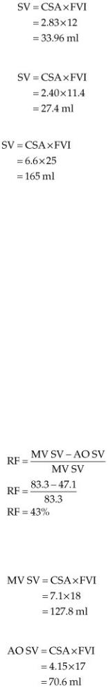
Aortic SV
Pulmonic SV
Mitral SV
Exercise 4-19 Answer
a)Calculate mitral stroke volume MV SV = CSA × FVI
MV SV = 4.9 × 17 MV SV = 83.3 ml
b)Calculate aortic stroke volume AO SV = CSA × FVI
AO SV = 3.14 × 15 AO SV = 47.1 ml
c)Calculate regurgitant fraction
In a normal heart with no leaking valves or shunts, the amount of blood flowing through each valve is equal. On a beat-to-beat basis, they may not be equal but over the course of several beats, volume will be similar. When there is mitral insufficiency, the extra volume flows through the mitral valve but not the aorta so the difference in volume between the two is equal to the regurgitant volume.
Exercise 4-20 Answer
a) Determine mitral stroke volume
b) Determine aortic stroke volume
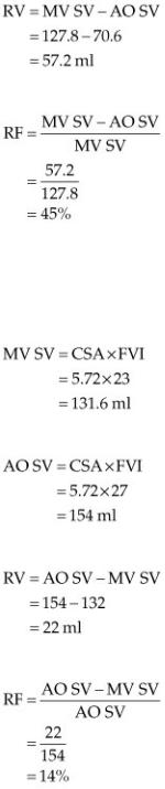
c)Calculate regurgitant volume
d)Calculate mitral regurgitant fraction
Exercise 4-21 Answer
Calculations:
a)Determine mitral stroke volume
b)Determine aortic stroke volume
c)Calculate aortic regurgitant volume
d)Calculate aortic regurgitant fraction
Exercise 4-22 Answer
a) Calculate pulmonary artery SV SV = CSA × FVI
SV = 4.15 cm2 × 28 cm SV = 116 ml
b) Calculate aortic SV SV = CSA × FVI
SV = 3.46 cm2 × 17 cm SV = 58.8 ml
c) Calculate Qp:Qs

Qp:Qs = PA SV/ AO SV Qp:Qs = 116/59
Qp:Qs = 2.0:1 d) Comments
Twice as much blood is flowing through the pulmonary circulation as the systemic circulation because of the shunt. Since there can be significant error built into the CSA measurements that can dramatically affect calculated shunt ratios, simply looking at peak flow velocities and flow integrals can provide information regarding the severity of the shunt. The higher the velocities and the larger the FVI the greater the volume flowing through that vessel. Normal PA FVI ranges from 7 to 19 cm. Since this puppy had PA FVI of 28 and a flow velocity of 2.9 m/sec, a significant shunt should be suspected. This only applies when there are no valvular insufficiencies at the flow sites interrogated.
Exercise 4-23 Answer
a)Calculate pulmonary artery SV
b)Calculate aortic SV
c)Calculate Qp:Qs
d)Comments
A shunt ratio of greater than 2.5 is considered to be very significant. FVI and peak velocities may be used in order to subjectively assess the severity of the shunt. Here the very high FVIs and peak velocities in the pulmonary artery suggest a hemodynamically significant shunt.
Exercise 4-24 Answer
a)Calculate pulmonary artery SV
b)Calculate aortic SV
c) Calculate Qp:Qs
d) Comments
The extra volume flowing through the lungs is recorded in the aorta before it shunts into the pulmonary artery and flow in the pulmonary artery is not increased until after the ductus enters it, beyond where Doppler flow is normally recorded. Therefore volume in the aorta is representative of flow that will go through the pulmonary circuit and flow in the pulmonary artery is representative of flow that will enter the systemic circulation. The shunt ratio is calculated in reverse compared to the other intracardiac shunts.

CHAPTER FIVE
Acquired Valvular Disease
The assessment of valvular insufficiency uses all echocardiographic modalities to assess the significance and severity of the leak. Two-dimensional and M–mode echocardiography are used to define valve morphology and structure including the type of lesion and the presence of valvular prolapse or ruptured chordae tendineae. Measurement of chamber size and function help define both the chronicity and the extent of remodeling.
Color-flow Doppler rapidly identifies the presence of regurgitation. Attention to the jet area with respect to the receiving chamber, the width of the jet at its orifice, and the area of flow convergence adds accuracy in assessing the severity of regurgitant volume. Spectral Doppler helps measure regurgitant volume and fraction and is used to measure regurgitant orifice area. Pulsed-wave Doppler and continuous-wave Doppler assess hemodynamic severity by evaluating spectral trace density, velocity of flows, and flow profiles (1).
Color-flow Doppler is notoriously variable if technical factors are not set properly. The color jet area of any regurgitation is inversely proportional to pulse repetition frequency (PRF and Nyquist limits), frame rates, and color gain. The size of the color jet area changes dramatically with different PRF settings. Increasing PRF will decrease the apparent size of a regurgitant jet and vice versa (Figure 5.1). The American Society of Echocardiography recommends setting the Nyquist limit between 50 and 60 cm/sec. Gain should be turned up to see color speckling and then turned back until speckling disappears (1). Using consistent and similar settings on the ultrasound equipment will help minimize errors in assessment and provide more accurate evaluation of changes over serial studies.
Color-Flow Settings for Regurgitation
Set gain just below level where speckle occurs.
Optimize frame rate.
Decrease 2D sector size.
Decrease color sector size.
Adjust packet size.
Adjust smoothing and frame averaging.
Jet area ↑ with ↓ PRF
Ideally set PRF to 50–60 cm/sec.
Figure 5.1 The size of the color jet area changes dramatically with different PRF settings. (A) Mitral regurgitation appears to fill the left atrium in this dog when the PRF is set at 53 cm/sec. (B) A PRF of 119 decreases the size of the regurgitant flow signal. LV = left ventricle, RV = right ventricle, RA = right atrium, LA = left atrium.