


3Relations; mappings; functions of a real variable
In this chapter, we deal with relations and a specification, namely mappings. Furthermore we introduce special mappings that are functions of one real variable, and we survey the most important types of functions of a real variable.
3.1 RELATIONS
A relation indicates a relationship between certain objects. A binary relation R from a set A to a set B assigns to each pair (a, b) A × B one of the two propositions:
(1)a is related to b by R, in symbols: aRb;
(2)a is not related to b by R, in symbols: aRb.
Definition 3.1 A (binary) relation R from a set A to a set B is a subset of the Cartesian
product A × B, i.e. R A × B.
We describe a relation R in one of the two following forms: (a, b) R aRb or R = {(a, b) A × B | aRb}. If R is a relation from set A to set A, we also say that R is a relation on A.
Example 3.1 Let us consider a relation R Z × Z on Z as follows. An integer i Z is related to integer j Z by R if and only if they have the same remainder when divided by 5. This means that e.g. 7 is related to 17 by R (i.e. 7R17) since both numbers give the remainder 2 when dividing by 5. Similarly, 9 is related to 4 by R (for both numbers, we get the remainder 4 when dividing them by 5), while 6 is not related to 13 (since 6 gives remainder 1, but 13 gives remainder 3) and 0 is not related to 23 (since 0 gives remainder 0, but 23 gives remainder 3). Moreover, relation R has the following two properties. First, every integer a is related to itself (i.e. aRa, such a relation is called reflexive), and relation R is symmetric, i.e. it always follows from aRb that bRa.
108 Relations; mappings; functions
Next, we give the notions of an inverse and a composite relation.
Definition 3.2 Let R A × B be a binary relation. Then the relation
R−1 = {(b, a) B × A | (a, b) R} B × A
(read: R inverse) is the inverse relation of R.
The following definition treats the case when it is possible to ‘concatenate’ two relations.
Definition 3.3 Let A, B, C be sets and R A × B, S B × C be binary relations. Then
S ◦ R = {(a, c) A × C | there exists some b B such that (a, b) R (b, c) S}
is called the composite relation or composition of R and S.
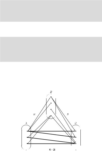
The composition of two relations is illustrated in Figure 3.1. The element a A is related to the element c C by the composite relation S ◦ R, if there exists (at least) one b B such that simultaneously a is related to b by R and b is related to c by S. We emphasize that the sequence of the relations in the composition is important, since the relations are described by ordered pairs. Therefore, in general S ◦ R = R ◦ S may hold, and one can interpret Definition 3.3 in such a way that first relation R and then relation S are used.
Figure 3.1 The composition S ◦ R.

Relations; mappings; functions 109
The following theorem gives a relationship between inverse and composite relations.
THEOREM 3.1 Let A, B, C be sets and R A × B and S B × C be binary relations. Then
(S ◦ R)−1 = R−1 ◦ S−1.
Theorem 3.1 is illustrated by the following example.
Example 3.2 Consider the relations |
|
|
R = {(x, y) R2 | y = ex} |
and |
S = {(x, y) R2 | x − y ≤ 2}. |
We apply Definition 3.3 and obtain for the possible compositions of both relations
S ◦ R = {(x, y) R2 | z R with z = ex z − y ≤ 2}
={(x, y) R2 | ex − y ≤ 2}
={(x, y) R2 | y ≥ ex − 2}
and
R ◦ S = {(x, y) R2 | z R with x − z ≤ 2 y = ez }
={(x, y) R2 | y > 0 z = ln y x − ln y ≤ 2}
={(x, y) R2 | y > 0 ln y ≥ x − 2}
={(x, y) R2 | y ≥ ex−2}.
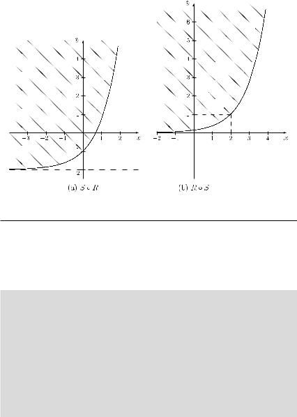
The graph of both composite relations is given in Figure 3.2. Moreover, we get
(S ◦ R)−1 = {(y, x) R2 | y ≥ ex − 2}, (R ◦ S)−1 = {(y, x) R2 | y ≥ ex−2}.
We now illustrate the validity of Theorem 3.1. Using
R−1 = {(y, x) R2 | y = ex},
S−1 = {(y, x) R2 | x − y ≤ 2},
we obtain
R−1 ◦ S−1 = {(y, x) R2 | z R with z − y ≤ 2 z = ex}
={(y, x) R2 | ex − y ≤ 2}
={(y, x) R2 | y ≥ ex − 2}
and
S−1 ◦ R−1 = {(y, x) R2 | z R with y = ez x − z ≤ 2}
={(y, x) R2 | y > 0 x − ln y ≤ 2}
={(y, x) R2 | y > 0 ln y ≥ x − 2}
={(y, x) R2 | y ≥ ex−2}.
110 Relations; mappings; functions
Figure 3.2 The compositions S ◦ R and R ◦ S in Example 3.2.
3.2 MAPPINGS
Next, we introduce one of the central concepts in mathematics.
Definition 3.4 Let A, B be sets. A relation f A × B, which assigns to every a A exactly one b B, is called a mapping (or a function) from set A into set B. We write
f : A → B
or, if the mapping is considered elementwise:
a A → f (a) = b B.
The set A is called the domain of the mapping, and the set B is called the target. For each a A, f (a) = b is called the image of a. The set of images of all elements of the domain is called the range f (A) B of the mapping.
A mapping associates with each element of A a unique element of B; the range f (A) may be a subset of B (see Figure 3.3). It follows from the above definition that a mapping is always

Relations; mappings; functions 111
Figure 3.3 Mapping f : A → B.
a relation, namely a particular relation R such that, for each a A, there is exactly one pair (a, b) A × B with (a, b) R. On the other hand, not every relation constitutes a mapping, e.g. the relation
R = {(x, y) R+ × R | x = y2}
is not a mapping. Indeed, for each x R+\{0}, there exist two values y = −√x and y2 = √x such that (x, y1) R and (x, y2) R (see Figure 3.4). 1
Figure 3.4 Relation R = {(x, y) R+ × R | x = y2}.
112 Relations; mappings; functions
Example 3.3 The German Automobile Association ADAC annually registers the breakdowns of most types of cars in Germany. For the year 2002, the following values (number of breakdowns per 10,000 cars of this type) for 10 types of medium-size cars with an age between four and six years have been obtained (see ADAC journal, May 2003): Toyota Avensis/Carina (TOY): 7.6, Mercedes SLK (MSLK): 9.1, BMW Z3 (BMWZ): 9.9, Mazda 626 (MAZ): 10.2, Mitsubishi Carisma (MIT): 12.0, Nissan Primera (NIS): 13.8, Audi A4/S4 (AUDI): 14.0, VW Passat (VW): 16.1, Mercedes C-class (MC): 17.5, BMW Series 3 (BMW3): 17.8. We should emphasize that we have presented the results only for the ten most reliable cars in this report among the medium-size cars.
Assigning to each car type the rank (i.e. the most reliable car gets rank one, the car in second place gets rank two and so on), we get a mapping f : Df → N with
Df = {TOY , MSLK, BMWZ, MAZ, MIT , NIS, AUDI , VW , MC, BMW 3}. Mapping f is given by f : {(TOY , 1), (MSLK, 2), (BMWZ, 3), (MAZ, 4), (MIT , 5), (NIS, 6), (AUDI , 7), (VW , 8), (MC, 9), (BMW 3, 10)}.
We continue with some properties of mappings.
Definition 3.5 A mapping f from A into B is called surjective if f (A) = B, i.e. for
each b B, there exists (at least) an a A such that f (a) = b.
A surjective mapping is also called an onto-mapping. This means that every element in set B is the image of some element(s) in set A.
Definition 3.6 A mapping f from A into B is called injective if for all a1, a2 A the following implication holds:
a1 = a2 f (a1) = f (a2)
(or equivalently, f (a1) = f (a2) a1 = a2).
This means that no two elements of set A are assigned to the same element of set B.
Definition 3.7 A mapping f from A into B is called bijective if f is surjective and
injective.
A bijective mapping is also called a one-to-one mapping. The notions of a surjective, an injective and a bijective mapping are illustrated in Figure 3.5.

Relations; mappings; functions 113
Figure 3.5 Relations and different types of mappings.
Example 3.4 Consider the following mappings:
f : R → R with f (x) = x2 g : N → N with g(x) = x2 h : R → R+ with h(x) = x2
k : R+ → R+ with k(x) = x2
Although we have the same rule for assigning the image f (x) to some element x for all four mappings, we get different properties of the mappings f , g, h and k. Mapping f is not injective since e.g. for x1 = −1 and x2 = 1, we get f (x1) = f (x2) = 1. Mapping f is also

114 Relations; mappings; functions
not surjective since not every y R is the image of some x Df = R. For instance, for y = −1, there does not exist an x R such that x2 = y.
Considering mapping g, we see that g is injective. For any two different integers x1 and x2, obviously the squares x12 and x22 are different, i.e. no two different natural numbers have the same image. However, mapping g is still not surjective since only squares of natural numbers
occur as image f (x). For instance, for y = 2, there does not exist a natural number x such that x2 = y.
Mapping h is surjective since for each y R+, there exists (at least) one x R such that f (x) = y, namely for x1 = √y (and for x2 = −√y, respectively), we get
f (x1) = (√y)2 = y (f (x2) = (−√y)2 = y).
Mapping h is not injective for the same reason that mapping f was not injective. Considering now mapping k, it is injective since any two different non-negative real numbers x1 and x2
have different squares: x2 = x2. Mapping k is also surjective since for any y R+, there
√ 1 2
exists an x = y ≥ 0, such that
f (x) = f (√y) = (√y)2 = y.
Therefore, mapping k is bijective.
Next, we define an inverse mapping and a composite mapping.
Definition 3.8 Let f : A → B be a bijective mapping. Then the mapping
f −1 : B → A
(read: f inverse) which assigns to any b B that a A with b = f (a), is called the inverse mapping of mapping f .
Definition 3.9 Let f : A → B and g : C → D be mappings with f (A) C. Then the mapping
g ◦ f : A → D,
which assigns to any a A a unique image (g ◦ f )(a) = g(f (a)) D, is called the composite mapping or composition of f and g.
The above definition reinforces the concept of a composite relation for the case of mappings. This means that for some a Df , mapping f is applied first, to give the image f (a). This image is assumed to be an element of the domain of mapping g, and we apply mapping g to f (a), yielding the image g(f (a)). It is worth emphasizing that, analogously to compositions

Relations; mappings; functions 115
of relations, the order of the sequence of the mappings in the notation g ◦ f is important, i.e. ‘g is applied after f ’.
Example 3.5 Consider the mappings f : A → A given by
{(1, 3), (2, 5), (3, 3), (4, 1), (5, 2)}
and g : A → A given by
{(1, 4), (2, 1), (3, 1), (4, 2), (5, 3)}.
For the ranges of the mappings we get
f (A) = {1, 2, 3, 5} |
and |
g(A) = {1, 2, 3, 4}. |
We consider the composite mappings f ◦ g and g ◦ f and obtain
(f ◦ g)(1) = f (g(1)) = f (4) = 1, (f ◦ g)(4) = f (2) = 5,
(g ◦ f )(1) = g(f (1)) = g(3) = 1, (g ◦ f )(4) = g(1) = 4,
(f ◦ g)(2) = f (1) = 3, (f ◦ g)(5) = f (3) = 3, (g ◦ f )(2) = g(5) = 3, (g ◦ f )(5) = g(2) = 1.
(f ◦ g)(3) = f (1) = 3,
(g ◦ f )(3) = g(3) = 1,
The composition g ◦ f is illustrated in Figure 3.6.
Figure 3.6 The composite mapping g ◦ f in Example 3.5.
For composite mappings g ◦ f , we have the following properties.
THEOREM 3.2 Let f : A → B and g : B → C be mappings. Then:
(1)If mappings f and g are surjective, mapping g ◦ f is surjective.
(2)If mappings f and g are injective, mapping g ◦ f is injective.
(3)If mappings f and g are bijective, mapping g ◦ f is bijective.

116 Relations; mappings; functions
Example 3.6 Consider the following mappings:
f : R → R with f (x) = 3x + 5; g : R → R with g(x) = ex + 1.
First, we show that both mappings f and g are injective. Indeed, for mapping f , it follows from x1 = x2 that 3x1 + 5 = 3x2 + 5. Analogously, for mapping g, it follows from x1 = x2 that ex1 + 1 = ex2 + 1. Then mapping g ◦ f with
(g ◦ f )(x) = g(f (x)) = g(3x + 5) = e3x+5 + 1
is injective as well due to part (2) of Theorem 3.2.
We can formulate a similar property for mappings as given in Theorem 3.1 for relations.
THEOREM 3.3 Let f : A → B and g : B → C be bijective mappings. Then the inverse mapping (f ◦ g)−1 exists, and we get
(f ◦ g)−1 = g−1 ◦ f −1.
Finally, we introduce an identical mapping as follows.
Definition 3.10 A mapping I : A → A with I (a) = a is called an identical mapping.
If for a mapping f : A → B the inverse mapping f −1 : B → A exists, then
f ◦ f −1 = f −1 ◦ f = I ,
where I is the identical mapping. This means that for each a A, we get
f ( f −1(a)) = f −1(f (a)) = a.
3.3 FUNCTIONS OF A REAL VARIABLE
In this section, we consider mappings or functions f : A → B with special sets A and B, namely both sets are either equal to the whole set R of real numbers or equal to a subset of R.

Relations; mappings; functions 117
3.3.1 Basic notions
Definition 3.11 A mapping f that assigns to any real number x Df R a unique real number y is called a function of a real variable. The set Df is called the domain of function f , and the set
Rf = f (Df ) = {y | y = f (x), x Df }
is called the range of function f .
We write y = f (x), x Df . Variable x is called the independent variable or argument, and y is called the dependent variable. The real number y is the image or the function value of x, i.e. the value of function f at point x. The domain and range of a function are illustrated in Figure 3.7.
Figure 3.7 Domain and range of a function f : Df → Rf .
We also write
f : Df → R or f : Df → Rf .
Alternatively we can also use the notation
f : {(x, y) | y = f (x), x Df }.
Hereafter, the symbol f denotes the function, and f (x) denotes the function value of a certain real number x belonging to the domain Df of function f . To indicate that function f depends on one variable x, one can also write f = f (x) without causing confusion.
A function f : Df → Rf can be represented analytically, graphically or in special cases by a table presenting for each point x Df the corresponding function value y = f (x) Rf .

118 Relations; mappings; functions
We can use the following analytical representations:
(1)explicit representation: y = f (x);
(2)implicit representation: F(x, y) = 0;
(3) parametric representation: x = g(t), y = h(t); t Dg = Dh.
In the latter representation, t is called a parameter which may take certain real values. For each value t Dg = Dh, we get a point (x, y) with y = f (x).
Example 3.7 Let function f : R → R be given in explicit form by
y = f (x) = x3 + 3x + 2.
The corresponding implicit representation is as follows:
F(x, y) = x3 + 3x + 2 − y = 0.
We emphasize that, from a given implicit or parametric representation, it is not immediately clear whether it is indeed a function (or only a relation).
Example 3.8 Consider the parametric representation |
|
||
x = r sin t, |
y = r cos t; |
t [0, 2π ]. |
(3.1) |
Taking the square of both equations and summing up, we get |
|
||
x2 + y2 = r2 · (sin2 t + cos2 t) = r2 |
|
||
which describes a circle with radius r and point (0, 0) as centre. Each point x |
(−r, r) |
||
is related to two values y1 = √r2 − x2 and y2 = −√r2 − x2. Therefore equation (3.1) characterizes only a relation.
The concept of bijective mappings can be immediately applied to a function of a real variable and we obtain: if a function f : Df → Rf , Df R, is bijective, then there exists a function f −1 which assigns to each real number y Rf a unique real value x Df with
x = f −1(y).
Here it should be mentioned that, if Rf R but Rf = R (in this case we say that Rf is a proper subset of R), the inverse function of f : Df → R would not exist, since f would not be surjective in that case. Nevertheless, such a formulation is often used and, in order to determine f −1, one must find the range Rf (in order to have a surjective mapping) or, equivalently, the domain Df −1 of the inverse function of f .

Relations; mappings; functions 119 We write f −1 : Rf → R or Rf → Df . Alternatively, we can use the notation
f −1 = {(y, x) | y = f (x), x Df }.
Since x usually denotes the independent variable, we can exchange variables x and y and write
y = f −1(x)
for the inverse function of function f with y = f (x). The graph of the inverse function f −1 is given by the mirror image of the graph of function f with respect to the line y = x. The graphs of both functions are illustrated in Figure 3.8. (In this case, function f is a linear function and the inverse function f −1 is linear as well.)
Figure 3.8 Graphs of functions f and f −1.
Example 3.9 Let function f : R+ → [4, ∞) with
y = f (x) = x3 + 4
be given. To determine the inverse function f −1, we solve the above equation for x and obtain
x3 = y − 4

120 Relations; mappings; functions
which yields
x = 3 y − 4.
Interchanging both variables, we obtain the inverse function
y = f −1(x) = |
√x − 4. |
||
|
3 |
|
|
The domain of the inverse function f −1 is the range of function f , and the range of function f −1 is the domain of function f , i.e.
Df −1 = [4, ∞) and Rf −1 = R+.
Analogously to our previous considerations in this chapter, we define composite functions of a real variable
g ◦ f : Df → R
with y = g(f (x)), x Df . Function f is called the inside function and function g is called the outside function. If there exists the inverse function f −1 for a function f , we have
f −1 ◦ f = f ◦ f −1 = I ,
i.e.
y = f −1(f (x)) = f (f −1(x)) = x,
where I is the identity function. We illustrate the concept of a composite function by the following examples.
Example 3.10 Let functions f : R → R and g : R → R with
f (x) = 3x − 2 and g(x) = x2 + x − 1
be given. We determine both composite functions f ◦ g and g ◦ f and obtain
(f ◦ g)(x) = f (g(x)) = f (x2 + x + 1) = 3(x2 + x − 1) − 2 = 3x2 + 3x − 5
and
(g ◦ f )(x) = g(f (x)) = g(3x − 2) = (3x − 2)2 + (3x − 2) − 1 = 9x2 − 9x + 1.
Both compositions are defined, since the range of the inside function is either set R (function f ) or a subset (function g) while in both cases the outside function is defined for all real numbers.

Relations; mappings; functions 121
Example 3.11 Given are the functions f : Df → R and g : Dg → R with
f (x) = √ |
|
|
Df = [−1, ∞) |
x + 1, |
|||
and |
|
||
g(x) = sin 3x, |
Dg = R. |
||
For the composite functions we obtain
( f ◦ g)(x) = f (g(x)) = f (sin 3x) = √sin 3x + 1
and
(g ◦ f )(x) = g(f (x)) = g(√x + 1) = sin(3√x + 1).
Composition f ◦ g is defined since the range Rg = [−1, 1] is a subset of the domain Df , and composition g ◦ f is defined since the range Rf = [0, ∞) is a subset of the domain Dg .
3.3.2 Properties of functions
Next, we discuss some properties of functions. We start with an increasing and a decreasing function.
Definition 3.12 A function f : Df → R is increasing (resp. strictly increasing) on an interval I Df if, for any choice of x1 and x2 in I with x1 < x2, inequality
f (x1) ≤ f (x2) (resp. f (x1) < f (x2))
holds.
Obviously, a strictly increasing function is a special case of an increasing function. The latter is also called a non-decreasing function in order to emphasize that there may be one or several subinterval(s) of I , where function f is constant.
Definition 3.13 A function f : Df → R is decreasing (resp. strictly decreasing) on an interval I Df if, for any choice of x1 and x2 in I with x1 < x2, inequality
f (x1) ≥ f (x2) (resp. f (x1) > f (x2))
holds.
A decreasing function is also called a non-increasing function. An illustration is given in Figure 3.9, where function f is strictly increasing on the interval I1, but strictly decreasing on the interval I2.
122 Relations; mappings; functions
Figure 3.9 Monotonicity of function f : Df → R.
We note that a function f : Df → Wf , which is strictly monotone on the domain (i.e. either strictly increasing on Df or strictly decreasing on Df , is bijective and therefore, the inverse function f −1 : Wf → Df exists in this case and is strictly monotone, too.
Example 3.12 We consider function f : Df → R with
2
f (x) = x + 1 .
This function is defined for all x = −1, i.e. Df = R \ {−1}. First, we consider the interval I1 = (−1, ∞). Let x1, x2 I1 with x1 < x2. We get 0 < x1 + 1 < x2 + 1 and thus
2 |
|
2 |
= f (x2). |
||
f (x1) = |
|
> |
|
||
x1 + 1 |
x2 + 1 |
||||
Therefore, function f |
is strictly decreasing on the interval I1. |
||||
Consider now the interval I2 = (−∞, −1) and let x1 < x2 < −1. In this case, we first get x1 + 1 < x2 + 1 < 0 and then
2 |
2 |
|
||
f (x1) = |
|
< |
|
= f (x2). |
x1 + 1 |
x2 + 1 |
|||
Therefore, function f is strictly increasing on the interval (−∞, −1). The graph of function f is given in Figure 3.10.

Relations; mappings; functions 123
Figure 3.10 Graph of function f in Example 3.12.
Definition 3.14 A function f : Df → R is said to be bounded from below (from above) if there exists a constant C such that
f (x) ≥ C (resp. f (x) ≤ C)
for all x Df . Function f is said to be bounded if f (x) is bounded from below and from above, i.e.
|f (x)| ≤ C
for all x Df .
Example 3.13 We consider function f : R → R with
y = f (x) = ex − 2.
Function f is bounded from below since f (x) ≥ −2 for all x R. However, function f is not bounded from above since f (x) can become arbitrarily large when x becomes large. Therefore, function f is not bounded.

124 Relations; mappings; functions
Example 3.14 We consider function f : R → R with
y = f (x) = 3 + sin 2x.
First, the function values of sin 2x are in the interval [−1, 1]. Therefore, the values of function f are in the interval [2, 4]. Consequently, for C = 4 we get |f (x)| ≤ C for all x R and thus, function f is bounded.
Definition 3.15 A function f : Df → R is called even (or symmetric) if
f (−x) = f (x).
Function f is called odd (or antisymmetric) if
f (−x) = −f (x).
In both cases, the domain Df has to be symmetric with respect to the origin of the coordinate system.
An even function is symmetric to the y-axis. An odd function is symmetric with respect to the origin of the coordinate system as a point. It is worth noting that a function f is not necessarily either even or odd.
Example 3.15 We consider function f : R \ {0} → R with
f (x) = 4x3 |
1 |
|
|
|
|
|
|
||
− 2x + |
|
. |
|
|
|
|
|
|
|
x |
|
|
|
|
|
||||
We determine f (−x) and obtain |
|
|
|
|
|
||||
f (−x) = 4(−x)3 − 2(−x) + |
1 |
= −4x3 |
1 |
||||||
|
+ 2x − |
|
|
||||||
−x |
x |
||||||||
= − |
4x3 − 2x + x |
= −f (x). |
|
|
|
||||
|
1 |
|
|
|
|
|
|
||
Thus, function f |
is an odd function. |
|
|
|
|
||||
Example 3.16 Let function f : R → R with
f (x) = 3x6 + x2

Relations; mappings; functions 125
be given. Then we obtain
f (−x) = 3(−x)6 + (−x)2 = 3x6 + x2 = f (x).
Hence, function f is an even function.
Definition 3.16 A function f : Df → R is called periodic if there exists a number T such that for all x Df with x + T Df , equality f (x + T ) = f (x) holds. The smallest real number T with the above property is called the period of function f .
Definition 3.17 A function f : Df → R is called convex (concave) on an interval I Df if, for any choice of x1 and x2 in I and 0 ≤ λ ≤ 1, inequality
f (λx1 + (1 − λ)x2) ≤ λf (x1) + (1 − λ)f (x2) |
(3.2) |
resp. f (λx1 + (1 − λ)x2) ≥ λf (x1) + (1 − λ)f (x2) |
(3.3) |
holds.
If for 0 < λ < 1 and x1 = x2, the sign < holds in inequality (3.2) (resp. the sign > in inequality (3.3)), function f is called strictly convex (strictly concave).
Figure 3.11 |
Illustration of a convex function f : Df |
→ R. |
The definition of a convex function is illustrated in Figure 3.11. Function f is convex on an interval I if for any choice of two points x1 and x2 from the interval and for any intermediate point x from the interval [x1, x2], which can be written as x = λx1 + (1 − λ)x2, the function

126 Relations; mappings; functions
value of this point (i.e. f (λx1 + (1 − λ)x2)) is not greater than the function value of the straight line through the points (x1, f (x1)) and (x2, f (x2)) at the intermediate point x. The latter function value can be written as λf (x1) + (1 − λ)f (x2).
Checking whether a function is convex or concave by application of Definition 3.17 can be rather difficult. In Chapter 4, we discuss criteria for applying differential calculus, which are easier to use. Here we consider, for illustration only, the following simple example.
Example 3.17 Let function f : R → R with
f (x) = ax + b
be given. Using formula (3.2) of the definition of a convex function, we obtain the following equivalences:
f (λx1 + (1 − λ)x2) ≤ λf (x1) + (1 − λ)f (x2)
a · [λx1 + (1 − λ)x2] + b ≤ λ · (ax1 + b) + (1 − λ) · (ax2 + b)
|
aλx1 + a(1 − λ)x2 + b |
≤ |
λax1 + λb + (1 − λ)ax2 + b − λb |
|
0 |
≤ |
0. |
Since the latter inequality is obviously true, the first of the above inequalities is satisfied too and hence, function f is convex. We mention that function f is also concave (all inequality signs above can be replaced by the sign ≥). So a linear function is obviously both convex and concave, but it is neither strictly convex nor strictly concave.
3.3.3 Elementary types of functions
Next, we briefly discuss some types of functions and summarize their main important properties. We start with polynomials and some of their special cases.
Polynomials and rational functions
Definition 3.18 The function Pn : R → R with
y = Pn(x) = anxn + an−1xn−1 + . . . + a2x2 + a1x + a0
with an = 0 is called a polynomial function (or polynomial) of degree n. The numbers a0, a1, . . . , an are called the coefficients of the polynomial.
Depending on the value of n which specifies the highest occurring power of x, we mention the following subclasses of polynomial functions:
n = 0 : |
y = P0 |
(x) = a0 |
|
constant function |
n = 1 : |
y = P1 |
(x) = a1x2+ a0 |
linear function |
|
n = 2 : |
y = P2 |
(x) = a2x3 |
+ a1x2+ a0 |
quadratic function |
n = 3 : |
y = P3 |
(x) = a3x |
+ a2x + a1x + a0 |
cubic function |
We illustrate the special cases of n = 1 and n = 2.

Relations; mappings; functions 127
Case n = 1 In this case, the graph is a (straight) line which is uniquely defined by any two distinct points P1 and P2 on this line. Assume that P1 has the coordinates (x1, y1) and P2 has the coordinates (x2, y2), then the above parameter a1 is given by
a1 = y2 − y1 x2 − x1
and is called the slope of the line. The parameter a0 gives the y-coordinate of the intersection of the line with the y-axis. These considerations are illustrated in Figure 3.12 for a0 > 0 and a1 > 0. The point-slope formula of a line passing through point P1 with coordinates (x1, y1) and having a slope a1 is given by
y − y1 = a1 · (x − x1).
Figure 3.12 A line with positive slope a1.
Example 3.18 Assume that for some product, the quantity of demand D depends on the price p as follows:
D = f (p) = 1, 600 − 1 · p. 2
The above equation describes the relationship between the price p of a product and the resulting demand D, i.e. it describes the amount of the product that customers are willing to purchase at different prices. The price p is the independent variable and demand D is the dependent variable. We say that f is the demand function. Since both price and demand can be assumed to be non-negative, we get the domain and range as follows:
Df = {p R | 0 ≤ p ≤ 3, 200} and Rf = {D R | 0 ≤ D ≤ 1, 600}.
If we want to give the price in dependence on the demand, we have to find the inverse function f −1 by solving the above equation for p. We obtain
1 · p = 1, 600 − D
2

128 Relations; mappings; functions
which corresponds to
p = f −1(D) = 2 · (1, 600 − D) = 3, 200 − 2D.
Here we did not interchange the variables since ‘D’ stands for demand and ‘p’ stands for price. Obviously, we get Df −1 = Rf and Rf −1 = Df .
Case n = 2 The graph of a quadratic function is called a parabola. If a2 > 0, then the parabola is open from above (upward parabola) while, if a2 < 0, then the parabola is open from below (downward parabola). A quadratic function with a2 > 0 is a strictly convex function while a quadratic function with a2 < 0 is a strictly concave function. The case of a downward parabola is illustrated in Figure 3.13. Point P is called the vertex (or apex), and its coordinates can be determined by rewriting the quadratic function in the following form:
y − y0 = a2 · (x − x0)2, |
|
|
|
|
|
|
|
|
(3.4) |
||||||||
where (x0, y0) are the coordinates of point P. We get |
|||||||||||||||||
x0 = − |
a1 |
|
and |
y0 = − |
|
a12 |
+ a0. |
||||||||||
2a2 |
|
4a2 |
|||||||||||||||
|
|
|
|
|
|
|
|
|
|
|
|
|
|
|
|
|
|
|
|
|
|
|
|
|
|
|
|
|
|
|
|
|
|
|
|
|
|
|
|
|
|
|
|
|
|
|
|
|
|
|
|
|
|
|
|
|
|
|
|
|
|
|
|
|
|
|
|
|
|
|
|
|
|
|
|
|
|
|
|
|
|
|
|
|
|
|
|
|
|
|
|
|
|
|
|
|
|
|
|
|
|
|
|
|
|
|
|
|
|
|
|
|
|
|
|
|
|
|
|
|
|
|
|
|
|
|
|
|
|
|
|
|
|
|
|
|
|
|
|
|
|
|
|
|
|
|
|
|
|
|
|
|
|
|
|
|
|
|
|
|
|
|
|
|
|
|
|
|
|
|
|
|
|
|
|
|
|
|
|
|
|
|
|
|
|
|
|
|
|
|
|
|
|
|
|
|
|
Figure 3.13 A downward parabola y = a2 · (x − x0)2 + y0.
Points x with y = f (x) = a2x2 + a1x + a0 = 0 are called the zeroes or roots of the quadratic function. In the case of a21 ≥ 4a2a0, a quadratic function has the two real zeroes
|
|
|
−a1 ± |
|
. |
|
x1,2 |
= |
a12 − 4a2a0 |
(3.5) |
|||
|
|
|||||
|
|
2a2 |
|
|||
In the case of a21 = 4a2a0, we get a zero x1 = x2 occurring twice. In the case of a21 < 4a2a0, there exist two zeroes which are both complex numbers. If a quadratic function is given in

Relations; mappings; functions 129
normal form y = x2 + px + q, formula (3.5) for finding the zeroes simplifies to
x1,2 = − p ± p2 − q.
24
Example 3.19 Consider the quadratic function P2 : R → R with
y = P2(x) = 2x2 − 4x + 4.
First, we write the right-hand side as a complete square and obtain
y = 2 · (x2 − 2x + 2) = 2 · (x − 1)2 + 2,
which can be rewritten as
y − 2 = 2 · (x − 1)2.
From the latter representation we see that the graph of function f is an upward parabola with the apex P = (1, 2) (see equation (3.4)). We investigate whether the inverse function f −1 exists. We try to eliminate variable x and obtain
y − 2 = (x − 1)2. 2
If we now take the square root on both sides, we obtain two values on the right-hand side, i.e.
|
|
|
|
|
= ± |
|
− |
|
|
|
|
|
|
|
|
|
||||||
2 |
|
|
|
|
|
|
|
|
|
|
|
|
||||||||||
|
|
|
y − 2 |
|
|
|
|
(x |
|
|
|
1) |
|
|
|
|
|
|
|
|
||
|
|
|
|
|
|
|
|
|
|
|
|
|
|
|
|
|
|
|||||
which yields the following two terms: |
|
|
|
|
|
|||||||||||||||||
|
1 |
= |
|
+ |
|
|
|
|
|
|
|
2 |
= |
|
− |
|
|
|
|
|||
|
|
|
|
2 |
|
|
|
|
|
2 |
|
|
||||||||||
x |
|
|
|
1 |
|
|
|
|
y |
− 2 |
|
and x |
|
|
1 |
|
|
y − 2 |
. |
|||
|
|
|
|
|
|
|
|
|
|
|
|
|
||||||||||
Therefore, the inverse function f −1 does not exist since the given function f is not injective.
If we restrict the domain of function f to the interval Df = [1, ∞), then the inverse function would exist since in this case, only solution x1 is obtained when eliminating variable x. Thus, we can now interchange both variables and obtain the inverse function f −1 with
|
= |
|
− |
|
= |
|
+ |
|
|
|
|
|
f − |
|
= [ |
|
∞ |
|
|
|
|
|
2 |
|
|
|
|
|
|
||||||||
y |
|
f |
|
1(x) |
|
1 |
|
|
x − 2 |
, |
D |
|
1 |
|
2, |
|
). |
|
|
|
|
|
|
|
|
|
|
||||||||||
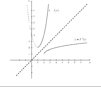
The graph of function f and the graph of the inverse function f −1 for the case when the domain of function f is restricted to Df = [1, ∞) are given in Figure 3.14.
130 Relations; mappings; functions
Figure 3.14 Graphs of functions f and f −1 in Example 3.19.
Next, we consider the general polynomial Pn of degree n with
Pn(x) = anxn + an−1xn−1 + · · · + a1x + a0, an = 0.
In the following, we give two properties of general polynomials and start with the fundamental theorem of algebra.
THEOREM 3.4 (fundamental theorem of algebra) Any polynomial Pn of degree n can be written as a product of polynomials of first or second degree.
Another important property of polynomials is given in the following remainder theorem. Let deg P denote the degree of polynomial P.
THEOREM 3.5 (remainder theorem) Let P : R → R and Q : with deg P ≥ deg Q. Then there always exist unique polynomials S such that
R → R be polynomials : R → R and R : R → R
P = S · Q + R, |
(3.6) |
where polynomial R is called the remainder and deg R < deg Q.

Relations; mappings; functions 131
If R(x) ≡ 0, then we say either that polynomial Q is a factor of polynomial P or that polynomial P is divisible by polynomial Q.
Consider the special case Q(x) = x − x0, i.e. polynomial Q is a linear function and we have deg Q(x) = 1. Then it follows from Theorem 3.5 that deg R = 0, i.e. R(x) = r is constant. This means that we can write polynomial P in the form
P(x) = S(x) · (x − x0) + r.
Consequently, for x = x0 we get the function value P(x0) = r. Furthermore, we have the following equivalence:
P(x) = S(x) · (x − x0) P(x0) = 0. |
(3.7) |
We can summarize the above considerations as follows. If x0 is a zero of a polynomial Pn with deg Pn = n (i.e. a root of the equation Pn(x) = 0), then, according to the comments above, this polynomial can be written as
Pn(x) = (x − x0) · Sn−1(x),
where Sn−1 is a polynomial with deg Sn−1 = n − 1. On the one hand, it follows from equivalence (3.7) that polynomial Pn can have at most n different zeroes. On the other hand, it follows from Theorem 3.4 that polynomial Pn has exactly n (real or complex) zeroes. If the polynomial Pn has the complex zero x = a + bi, then the complex conjugate x = a − bi
is a zero of polynomial Pn, too. Therefore, polynomial Pn has the factors
x − (a + bi) · x − (a − bi) = x2 − 2ax + (a2 + b2),
which is a polynomial of degree two. So we can confirm Theorem 3.4. A real zero x0 leads to a polynomial x − x0 of first degree and complex zeroes a + bi and a − bi to a polynomial x2 − 2ax + (a2 + b2) of second degree in the product representation of polynomial Pn. As a consequence of the above considerations, we can conclude for example that a polynomial P3 of degree three has either three real zeroes or only one real zero (and two complex zeroes).
It may happen that certain factors x − xi occur repeatedly in the above representation. This leads to the definition of the multiplicity of a zero.
Definition 3.19 Let f = Pn : R → R be a polynomial of degree n with
Pn(x) = (x − x0)k · Sn−k (x) |
and |
Sn−k (x0) = 0. |
Then x0 is called a zero (or root) of multiplicity k of polynomial Pn.
If x0 is a zero of odd multiplicity, then the sign of function f changes ‘at’ point x0, i.e. there exists an interval about x0 such that function f has positive values to the left of x0 and negative values to the right of x0 or vice versa. In contrast, if x0 is a zero of even multiplicity, there is an interval about x0 such that the sign of function f is the same on both sides of point x0.
Next, we investigate the question of how to compute the function value of a polynomial easily. To this end, we introduce Horner’s scheme.
132 Relations; mappings; functions
Calculation of function values of polynomials using Horner’s scheme
P |
(x |
) |
= |
a xn |
+ |
a |
n−1 |
xn−1 |
+ · · · + |
a |
x2 |
+ |
a |
x |
0 |
+ |
a |
0 |
||||||||
n |
0 |
|
|
n 0 |
|
|
|
0 |
|
2 |
0 |
1 |
|
|
||||||||||||
= { · · · [(anx0 |
|
+ an−1) x0 + an−2] x0 + · · · + a1} x0 + a0 |
||||||||||||||||||||||||
|
|
|
|
|
|
|
|
|
An |
2 |
|
|
|
|
|
|
|
|
|
|
|
|
|
|||
|
|
|
|
|
|
An−1 |
|
|
|
|
|
|
|
|
|
|
|
|
|
|
|
|
||||
|
|
|
|
|
|
|
|
|
|
|
|
A1 |
|
|
|
|
|
|
|
|
|
|
||||
|
|
|
|
|
|
|
|
|
|
|
− |
|
|
|
|
|
|
|
|
|
|
|
|
|
||
|
|
|
|
|
|
|
|
|
|
|
|
|
|
|
|
|
|
|
|
|
|
|
|
|||
The above computations can be easily performed using the following scheme and starting from the left.
Horner’s scheme |
|
|
|
|
|
|
|
|
||
|
|
an |
an−1 |
an−2 |
. . . |
a2 |
a1 |
a0 |
||
|
|
|||||||||
|
x = x0 |
|
+ |
+ |
|
+ |
+ |
+ |
|
|
|
|
anx0 |
An−1x0 . . . |
A3x0 |
A2x0 |
A1x0 |
||||
|
|
|
|
|
|
|
|
|
|
|
|
|
an |
An−1 |
An−2 . . . |
A2 |
A1 |
A0 = Pn(x0) |
|||
|
|
|
|
|
|
|
|
|
|
|
The advantage of Horner’s scheme is that, in order to compute the function value of a polynomial, only additions and multiplications have to be performed, but it is not necessary to compute powers.
Example 3.20 We consider the polynomial P5 : R → R with
P5(x) = 2x5 + 4x4 + 8x3 − 4x2 − 10x.
Since a0 = 0, we get the zero x0 = 0 and dividing P4(x) by x − x0 = x yields the polynomial P4 with
P4(x) = 2x4 + 4x3 + 8x2 − 4x − 10.
Checking now the function values for x2 = 1 and x3 = −1 successively by Horner’s scheme, we obtain
x = x2 = 1 |
2 |
4 |
8 |
−4 |
−10 |
|
2 |
6 |
14 |
10 |
|
x = x3 = −1 |
2 |
6 |
14 |
10 |
0 |
|
−2 −4 −10 |
|
|||
|
2 |
4 |
10 |
0 |
|
In the above scheme, we have dropped the arrows and the plus signs for simplicity. We have found that both values x2 = 1 and x3 = −1 are zeroes of the polynomial P4(x). From the last row we see that the quadratic equation 2x2 + 4x + 10 = 0 has to be considered to determine the remaining zeroes of polynomial P4. We obtain
x4,5 = −1 ± √1 − 5

Relations; mappings; functions 133
which yields the complex zeroes
x4 = −1 + 2i and x5 = −1 − 2i.
So we have found all five (real and complex) zeroes of polynomial P5(x), and we get the factorized polynomial
P5(x) = 2x(x − 1)(x + 1)(x2 + 2x + 5).
Example 3.21 We consider the polynomial P5 : R → R with
P5(x) = x5 − 5x4 + 40x2 − 80x + 48
and determine the multiplicity of the (guessed) zero x = 2. We obtain:
x = 2 |
1 |
−5 |
0 |
40 |
−80 |
48 |
|
2 |
−6 −12 |
56 |
−48 |
||
x = 2 |
1 |
−3 |
−6 |
28 |
−24 |
0 |
|
2 |
−2 |
−16 |
24 |
|
|
x = 2 |
1 |
−1 |
−8 |
12 |
0 |
|
|
2 |
2 |
−12 |
|
|
|
x = 2 |
1 |
1 |
−6 |
0 |
|
|
|
2 |
6 |
|
|
|
|
|
1 |
3 |
0 |
|
|
|
Thus, x = 2 is a zero of multiplicity four, and the polynomial P5 can be written as a product as follows:
P5(x) = (x − 2)4 · (x + 3).
The last factor is obtained from the remaining polynomial S1 with S1(x) = x + 3 which has the zero x = −3.
In general, it is difficult to find all zeroes of a polynomial of a higher degree. In Chapter 4, we discuss numerical procedures for finding the zeroes approximately. The following theorem gives some relationships between the coefficients of a polynomial and the zeroes.
THEOREM 3.6 (Vieta’s theorem) Let polynomial Pn : R → R with
Pn(x) = 1 · xn + an−1xn−1 + · · · + a2x2 + a1x + a0

134 Relations; mappings; functions
be given and let x1, x2, · · · , xn be the zeroes of polynomial Pn. Then:
x1 + x2 + · · · + xn |
= −an−1 |
|
x1x2 + x1x3 + · · · + xn−1xn |
= |
an−2 |
x1x2x3 + x1x2x4 + · · · + xn−2xn−1xn |
= −an−3 |
|
. |
|
. |
. |
|
. |
. |
|
. |
x1x2x3 · · · xn |
= (−1)na0 |
|
In the special case of a quadratic function P2(x) = x2 + px + q, Vieta’s theorem yields the two equations
x1 + x2 = −p and x1x2 = q.
Example 3.22 Let the polynomial P3 : R → R with
P3(x) = x3 − 2x2 − 5x + 6
be given. When looking for integer zeroes, it follows from the last equality of Theorem 3.6 that these zeroes must be a divisor of a0 = 6. Therefore, only x = ±1, x = ±2 and x = ±3 are candidates for an integer zero. Checking the function values of P3 at these points e.g. by Horner’s scheme, we obtain the zeroes
x1 = 1, x2 = −2 and x3 = 3
and thus the factorized polynomial
P3 = (x − 1) · (x + 2) · (x − 3).
Finally, we consider the quotient of two polynomials, P and Q.
Definition 3.20 A function T : DT → R with T (x) = P(x)/Q(x) = (P/Q)(x) is called a rational function. The rational function T is called proper if deg P < deg Q and improper if deg P ≥ deg Q.
The domain DT of function T is given by all real numbers for which the polynomial in the denominator is different from zero, i.e. DT = {x R | Q(x) = 0}.
Example 3.23 Let the cost C of producing x units of a product be equal to
C(x) = ax2 + bx + c, x ≥ 0.
Here c > 0 describes the fixed cost of production, and a and b are real parameters such that C is a non-negative and strictly increasing function. Then the average cost Ca(x), measuring

Relations; mappings; functions 135
the cost per unit produced, given by
Ca(x) = ax2 + bx + c x
is an improper rational function which can be rewritten as
Ca(x) = ax + b + c . x
By means of polynomial division, any improper rational function can be written as the sum of a polynomial and a proper rational function. If deg P ≥ deg Q, then equation (3.6) can be written as
P(x) = S(x) + R(x)
Q(x) Q(x)
provided that x is not a zero of polynomial Q. To get the latter representation, we consider both polynomials P and Q in decreasing order of their powers and divide in each step the first term of P by the first term of Q. The result is multiplied by Q and the product is then subtracted from P. This yields a new polynomial P1 having a smaller degree than polynomial Pn. Now the first term (with the largest exponent) of polynomial P1 is divided by the first term of polynomial Q, the resulting term is multiplied by polynomial Q and subtracted from P1, yielding polynomial P2 and so on. The procedure stops if some resulting polynomial Pi has a smaller degree than polynomial Q. This procedure is illustrated by the following example.
Example 3.24 Let polynomials P : R → R and Q : R → R with
P(x) = 2x4 − 3x3 + 2x2 − x + 4 and Q(x) = x2 − x + 3
be given. The function T : DT → R with T (x) = (P/Q)(x) is improper, and by polynomial division we obtain:
(2x4 |
− |
3x3 |
+ |
2x2 |
− |
x |
+ |
4) : (x2 |
|
|
|
|
|
|
|
|
|
|
|
x2 |
x 3 |
|
|
|
|
|
− |
x |
+ |
3) |
= |
2x2 |
− |
x |
− |
5 |
+ |
−3x+19 |
|||||||
−(2x4 − 2x3 + 6x2) |
|
|
|
|
|
|
|
|
|
|
|
− + |
||||||||||
|
|
−x3 |
− 4x2 − |
x + 4 |
|
|
|
|
|
|
|
|
|
|
|
|
|
|||||
|
|
3 |
|
2 |
|
|
|
|
|
|
|
|
|
|
|
|
|
|
|
|
|
|
|
− (−x |
+ x |
− 3x) |
|
|
|
|
|
|
|
|
|
|
|
|
|
|
|
|
|||
|
|
|
|
−5x2 |
+ 2x + |
4 |
|
|
|
|
|
|
|
|
|
|
|
|
|
|
||
−(−5x2 + 5x − 15)
−3x + 19
In this case, we have written function T as the sum of the polynomial S of degree two with S(x) = 2x2 − x − 5 and the proper rational function R/Q with
(R/Q)(x) = (−3x + 19)/(x2 − x + 3).

136 Relations; mappings; functions
Power functions
Definition 3.21 The function f : Df → R with
f (x) = xr , |
r R, |
is called a power function. In dependence on the value of r, the domain Df and the range Rf are given as follows:
(1)r {1, 3, 5, . . .} N : Df = (−∞, ∞), Rf = (−∞, ∞);
(2)r {2, 4, 6, . . .} N : Df = (−∞, ∞), Rf = [0, ∞);
(3)r R \ N : Df = (0, ∞), Rf = (0, ∞).
In case (1), function f is strictly increasing, unbounded and odd. Function f is strictly concave on the interval (−∞, 0] and strictly convex on the interval [0, ∞). In case (2), function f is strictly decreasing on the interval (−∞, 0], strictly increasing on the interval [0, ∞), bounded from below, even and strictly convex. Since function f is not injective in this case (note that f (−x) = −f (x)), the inverse function does not exist in this case (if one restricts the domain to the interval [0, ∞), then function f is bijective and the inverse function exists). In case (3) with r > 0, function f is strictly increasing and bounded from below. Moreover, if r > 1, function f is strictly convex and, if 0 < r < 1, function f is strictly concave. Case (3) with positive value r includes as a special case so-called root functions, where r = 1/n with n N, i.e.
√
f (x) = x1/n = n x.
In the case of a root function, number zero belongs to the domain and range of f , i.e. Df = Rf = [0, ∞). In case (3) with r < 0, function f is strictly decreasing, bounded from below and strictly convex.
Obviously, the inverse function f −1 of a power function f with f (x) = xr exists and is equal to y = x1/r . The graph of some power functions for special values of r are given in Figure 3.15. If r Q, we say that power function f is an algebraic function.
Example 3.25 Let function f : (0, ∞) → (0, ∞) with
f (x) = x2.5
be given. It is a power function with the rational exponent r = 2.5. This function is bijective, and so the inverse function exists. Solving for variable x, we obtain
x = y1/2.5 = y0.4.
Exchanging both variables x and y, we get the inverse function f −1 with
y = x0.4, Df −1 = Rf = (0, ∞).

Relations; mappings; functions 137
Figure 3.15 Graphs of some power functions.
Exponential and logarithmic functions
Exponential and logarithmic functions play an important role in many economic applications, e.g. growth and decline processes.
Definition 3.22 The function f : R → (0, ∞) with
f (x) = ax, a > 0, a = 1,
is called an exponential function.

138 Relations; mappings; functions
For all positive values of a, the graph of function f goes through point (0, 1). The graph of the exponential function for three values of a is given in Figure 3.16. For all values of a, the exponential function is only bounded from below (and therefore unbounded). If a > 1, the exponential function is strictly increasing, while for 0 < a < 1 the exponential function is strictly decreasing. All exponential functions are strictly convex. We note that for an exponential function with base e, the notation y = ex is sometimes also written as y = exp(x).
Since an exponential function f is bijective for all values a > 0 with a = 1 on the domain Df , for each of these values of a the inverse function exists. The inverse function of the exponential function is the logarithmic function defined as follows.
Figure 3.16 Graphs of some exponential functions.
Definition 3.23 The function f : (0, ∞) → R with
f (x) = loga x, a > 0, a = 1,
is called a logarithmic function.
Relations; mappings; functions 139
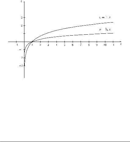
Figure 3.17 Graphs of some logarithmic functions.
The graphs of the logarithmic functions with the two frequently used bases a = e and a = 10 are given in Figure 3.17. Since the logarithmic functions are the inverse functions of the corresponding exponential functions, all logarithmic functions go through the point (1,0). Logarithmic functions with a base a > 1 are strictly increasing, and logarithmic functions with a base a, where 0 < a < 1, are strictly decreasing. All logarithmic functions are unbounded. Logarithmic functions with a base a > 1 are strictly concave while logarithmic functions with a base a, where 0 < a < 1, are strictly convex. It is worth emphasizing that both logarithmic and exponential functions are only defined for positive values of the base, where a base equal to one is excluded.
Example 3.26 We consider function f : Df → R with
y = f (x) = ln(3x + 4).
Since the logarithmic function is defined only for positive arguments, the inequality 3x+4 > 0 yields the domain
Df = |
x R | x > − |
4 |
. |
3 |
The logarithmic function has the range Rf = R, and therefore function f also has the range Rf = R. Since the logarithmic function is bijective, function f is bijective as well, and thus

140 Relations; mappings; functions
the inverse function f −1 exists. We obtain
y = ln(3x + 4)
ey = 3x + 4
x= 1 · ey − 4 . 3
Exchanging now variables x and y, we have found the inverse function f −1 given by
y = 1 · (ex − 4)
3
with the domain Df −1 = Rf = R.
Trigonometric functions
Trigonometric (or circular) functions are defined by means of a circle with the origin as centre and radius r (see Figure 3.18). Let P be the point on the circle with the coordinates (r, 0) and assume that this point moves now counterclockwise round the circle. For a certain angle x, we get a point P on the circle with the coordinates (h, v). Then the sine and cosine functions are defined as follows.
Figure 3.18 The definition of the trigonometric functions.

Relations; mappings; functions 141
Definition 3.24 The function f : R → [1, 1] with
f (x) = sin x = v r
is called the sine function. The function f : R → [1, 1] with
f (x) = cos x = h r
is called the cosine function.
The graphs of the sine and cosine functions are given in Figure 3.19 (a). The sine and cosine functions are bounded and periodic functions with a period of 2π , i.e. we have for k Z:
sin(x + 2kπ ) = sin x and |
cos(x + 2kπ ) = cos x. |
The sine function is odd, while the cosine function is even. These functions are often used to model economic cycles.
Remark Usually, angles are measured in degrees. Particularly in calculus, they are often measured in so-called radians (abbreviated rad). An angle of 360◦ corresponds to 2π rad, i.e. we get for instance
sin 360◦ = sin 2π rad.
It is worth noting that, using radians, the trigonometric functions have set R or a subset of R as domain and due to this, the abbreviation rad is often skipped.
When using powers of trigonometric functions, we also write e.g. sin2 x instead of (sin x)2 or cos3(2x) instead of (cos 2x)3. By means of the sine and the cosine functions, we can introduce two further trigonometric functions as follows.
Definition 3.25 The function f : Df → R with |
|
|
||||||||||
f (x) = tan x = |
|
sin x |
= |
|
v |
and |
Df = *x R | x = |
π |
+ kπ , k Z+ |
|||
|
|
|
|
|
|
|
||||||
cos x |
h |
2 |
||||||||||
is called the tangent function. The function f : Df → R with |
|
|
||||||||||
|
|
cos x |
|
|
h |
|
|
|
|
|||
f (x) = cot x = |
|
|
= |
|
|
and |
Df = {x R | x = kπ , k Z} |
|||||
sin x |
|
v |
||||||||||
is called the cotangent function.
142 Relations; mappings; functions
Figure 3.19 Graphs of the trigonometric functions.
The graphs of the tangent and cotangent functions are given in Figure 3.19 (b). The tangent and cotangent functions are periodic functions with a period of π , i.e. we have for k Z:
tan(x + kπ ) = tan x and |
cot(x + kπ ) = cot x. |
Both functions are unbounded and odd.
In the following, we review some basic properties of trigonometric functions.
Some properties of trigonometric functions
(1)sin(x ± y) = sin x cos y ± cos x sin y;
(2)cos(x ± y) = cos x cos y sin x sin y;
(3) tan(x y) |
|
tan x ± tan y |
; |
||
|
|
||||
± |
= |
1 |
|
tan x tan y |
|
|
|
||||

Relations; mappings; functions 143
(4) |
cot(x |
± |
y) |
= |
|
cot x cot y 1 |
; |
|
|
||||
|
|
||||||||||||
|
|
|
|
cot y |
± |
cot x |
|||||||
|
|
|
|
|
|
|
x ± y |
|
|
x y |
|
||
(5) |
sin x ± sin y = 2 · sin |
· cos |
; |
||||||||||
|
|
||||||||||||
22
(6)cos x + cos y = 2 · cos x + y · cos x − y ;
|
|
|
|
|
|
|
|
|
2 |
+ y |
|
2 |
|
|
|
|||
cos x |
− |
cos y |
= − |
2 |
· |
sin |
x |
· |
sin |
x − y |
; |
|||||||
|
|
|
|
|||||||||||||||
|
|
|
|
|
|
|
|
2 |
|
2 |
|
|
||||||
(7) sin x ± |
π |
|
|
|
|
|
|
|
|
|
|
π |
= sin x; |
|||||
|
|
= ± cos x, |
|
cos x ± |
|
|||||||||||||
2 |
|
2 |
||||||||||||||||
= 1; 1
cos2 x .
Properties (1) up to (4) are known as addition theorems of the trigonometric functions. For the special case of x = y, properties (1) and (2) turn into
sin 2x = 2 · sin x · cos x |
and |
cos 2x = cos2 x − sin2 x. |
(3.8) |
Property (8) is also denoted as a Pythagorean theorem for trigonometric functions. As an illustration, we prove the identity given in Property (9) and obtain
1 |
+ |
tan2 x |
|
1 |
|
sin2 x |
|
cos2 x + sin2 x |
|
1 |
. |
= |
+ cos2 x |
= |
cos2 x |
|
|||||||
|
|
|
= cos2 x |
||||||||
The last equality follows from property (8) above.
Since all four trigonometric functions are not bijective mappings, we have to restrict their domain in order to be able to define inverse functions. If we solve equality y = sin x for x, we write x = arcsin y. The term arcsin y gives the angle x whose sine value is y. Similarly, we use the symbol ‘arc’ in front of the other trigonometric functions when solving for x. Now we can define the arc functions as follows.
Definition 3.26 The function |
|
||||||||||
|
π |
π |
|
|
|
|
|||||
f |
: [−1, 1] → − |
|
, |
|
|
|
|
with f (x) = arcsin x |
|||
2 |
2 |
||||||||||
is called the arcsine function. The function |
|||||||||||
f |
: [−1, 1] → [0, π ] |
|
|
|
|
with |
f (x) = arccos x |
||||
is called the arccosine function. The function |
|||||||||||
f |
: (−∞, ∞) → − |
π |
|
π |
|
with f (x) = arctan x |
|||||
|
, |
|
|
||||||||
2 |
2 |
||||||||||
is called the arctangent function. The function |
|||||||||||
f |
: (−∞, ∞) → (0, π ) |
|
|
with |
f (x) = arccot x |
||||||
is called the arccotangent function.

144 Relations; mappings; functions
In Definition 3.26, the ranges of the arc functions give the domains of the original trigonometric functions such that they represent bijective mappings and an inverse function can be defined. The graphs of the arc functions are given in Figure 3.20. All the arc functions are bounded. The arcsine and arctangent functions are strictly increasing and odd while the arccosine and arccotangent functions are strictly decreasing. Moreover, the arcsine and arccotangent functions are strictly concave for x ≤ 0 and they are strictly convex for x ≥ 0. The arccosine and arctangent functions are strictly convex for x ≤ 0 and strictly concave for x ≥ 0 (where in all cases, x has to belong to the domain of the corresponding function).
Figure 3.20 Graphs of the inverse functions of the trigonometric functions.

Relations; mappings; functions 145
Overview on elementary functions
In Table 3.1, we summarize the domains and ranges of the elementary functions.
Table 3.1 Domains and ranges of elementary functions
Function f with |
y = f (x) |
Df |
|
|
|
|
Rf |
|
|
|
|
|
|
|
|
|
|
|||||||
y = cn |
c is constant |
−∞ < x < ∞ |
|
|
|
y = c |
|
|
|
|
||||||||||||||
y = xα |
n = 2, 3, . . . |
−∞ < x < ∞ −∞ < y < ∞ |
||||||||||||||||||||||
y = xn |
|
|
α R |
0 < x < ∞ 0 < y < ∞ |
||||||||||||||||||||
|
||||||||||||||||||||||||
y |
= |
|
x |
n |
= |
2, 3, . . . |
0 |
≤ |
x < |
∞ |
|
0 |
≤ |
y < |
∞ |
|||||||||
|
√x |
|
|
|
|
|
|
|
|
|
|
|||||||||||||
y = a |
|
|
|
a > 0 |
−∞ < x < ∞ 0 < y < ∞ |
|||||||||||||||||||
y = loga x |
a > 0, a = 1 0 < x < ∞ |
−∞ < y < ∞ |
||||||||||||||||||||||
y = sin x |
|
|
|
−∞ < x < ∞ |
−1 ≤ y ≤ 1 |
|||||||||||||||||||
y |
= |
cos x |
|
|
|
−∞ π |
|
∞ |
− |
1 |
≤ |
y |
≤ |
1 |
|
|||||||||
|
|
|
|
|
< x < |
|
|
|
|
|
|
|||||||||||||
y = tan x |
|
|
|
x = |
|
+ k π |
−∞ < y < ∞ |
|||||||||||||||||
|
|
|
2 |
|||||||||||||||||||||
y = cot x |
|
|
|
x = k π |
|
−∞π |
< y < ∞π |
|||||||||||||||||
y = arcsin x |
|
|
|
−1 ≤ x ≤ 1 |
− |
|
|
≤ x ≤ |
|
|
|
|
||||||||||||
|
|
|
2 |
|
2 |
|
||||||||||||||||||
y |
= |
arccos x |
|
|
|
−1 ≤ x ≤ 1 |
|
π0 |
≤ x ≤ |
|
π |
|||||||||||||
|
|
|
|
|
|
|
|
|
|
|
|
|
|
|
|
π |
||||||||
y = arctan x |
|
|
|
−∞ < x < ∞ |
− |
|
|
< x < |
|
|
|
|||||||||||||
|
|
|
2 |
|
2 |
|
||||||||||||||||||
y = arccot x |
|
|
|
−∞ < x < ∞ |
|
|
0 < x < π |
|||||||||||||||||
EXERCISES
3.1Let A = {1, 2, 3, 4, 5}. Consider the relations
R = {(1, 2), (1, 4), (3, 1), (3, 4), (3, 5), (5, 1), (5, 4)} A × A
and
S = {(a1, a2) A × A | a1 + a2 = 6}.
(a)Illustrate R and S by graphs and as points in a rectangular coordinate system.
(b)Which of the following propositions are true of relation R:
1R2, 2R1, 3R1, {2, 3, 4, 5} = {a A | 1Ra}?
(c)Find the inverse relations for R and S.
(d)Check whether the relations R and S are mappings.
146Relations; mappings; functions
3.2Consider the following relations and find out whether they are mappings. Which of the mappings are surjective, injective, bijective?
(a)
a 1 |
|
b |
2 |
|
|
c |
|
3 |
|
(b) |
|
|
|
|
|
(c) |
|
|
|
(d) |
|
|
|
|
|
a |
|
|
|
a |
|
|
|
1 |
1 |
|
a |
||||
c |
|
|
|
||||||||||||
|
|
b |
|
|
|
|
|
|
|||||||
3 |
|
|
|
|
2 |
3 |
|
|
b |
||||||
|
|
|
|
|
|
|
|
|
|
|
|
|
|
||
|
|
|
|
|
|
|
|
|
|
|
|
|
|||
5 |
|
|
|
|
f |
c |
|
|
|
4 |
5 |
|
|
c |
|
|
|
|
|
|
|
|
|
|
|||||||
|
|
|
|
|
|
|
|
|
|
6 |
7 |
|
|
d |
|
|
|
|
|
|
|
|
|
|
|
|
|
|
g |
||
|
|
|
|
|
|
|
|
|
|
|
|
|
|
||
3.3Let A = B = {1, 2, 3} and C = {2, 3}. Consider the following mappings f : A → B and g : C → A with f (1) = 3, f (2) = 2, f (3) = 1 and g(2) = 1, g(3) = 2.
(a)Illustrate f , g, f ◦ g and g ◦ f by graphs if possible.
(b)Find the domains and the ranges of the given mappings and of the composite mappings.
(c)What can you say about the properties of these mappings?
3.4Given is the relation
F = {(x1, x2) R2 | |x2| = x1 + 2}.
Check whether F or F−1 is a mapping. In the case when there is a mapping, find the domain and the range. Graph F and F−1.
3.5Given are the relations
F = {(x1, x2) | x2 = x13} with x1 {−3, −2, −1, 0, 1, 2, 3}
and
G = {(x, y) R2 | 9x2 + 2y2 = 18}.
Are these relations functions? If so, does the inverse function exist? 3.6 Given are the functions f : Df → R and g : Dg → R with
f (x) = 2x + 1 and g(x) = x2 − 2.
Find and graph the composite functions g ◦ f and f ◦ g.
3.7Given are the functions f : R → R+ and g : R → R with
f (x) = ex and g(x) = −x.
(a)Check whether the functions f and g are surjective, injective or bijective. Graph these functions.
(b)Find f −1 and g−1 and graph them.
(c)Find f ◦ g and g ◦ f and graph them.
|
|
|
|
|
|
|
|
|
|
Relations; mappings; functions 147 |
3.8 |
Find a R such that f : Df |
= [a, ∞) → R with |
||||||||
|
y = f (x) = x2 + 2x − 3 |
|
|
|
|
|||||
|
being a bijective function. Find and graph function f −1. |
|||||||||
3.9 |
Find domain, range and the inverse function for function f : Df → R with y = f (x): |
|||||||||
|
|
√ |
|
|
|
|
= |
|
− |
|
|
|
= √x + 4 |
|
|
|
|
||||
|
(a) y |
|
x |
− 4 ; |
(b) |
y |
|
(x |
|
2)3. |
|
|
|
|
|
||||||
3.10Given are the polynomials P5 : R → R and P2 : R → R with
P5(x) = 2x5 − 6x4 − 6x3 + 22x2 − 12x and P2(x) = (x − 1)2.
(a)Calculate the quotient P5/P2 by polynomial division.
(b)Find all the zeroes of polynomial P5 and factorize P5.
(c)Verify Vieta’s formulae given in Theorem 3.6.
(d)Draw the graph of the function P5.
3.11Check by means of Horner’s scheme whether x1 = 1, x2 = −1, x3 = 2, x4 = −2 are zeroes of the polynomial P6 : R → R with
P6(x) = x6 + 2x5 − x4 − x3 + 2x2 − x − 2.
Factorize polynomial P6.
3.12Find the domain, range and the inverse function for each of the following functions fi : Dfi → R with yi = fi(x):
(a) |
y1 |
= sin x, |
y2 = 2 sin x, y3 = sin 2x, y4 = sin x + 2 |
and |
|
y5 |
= sin(x + 2); |
y5 = e x+2. |
|
(b) |
y1 |
= e x, |
y2 = 2e x, y3 = e2x, y4 = e x + 2 and |
|
Graph the functions given in (a) and (b) and check whether they are odd or even or whether they have none of these properties.
3.13Given are the following functions f : Df → R with y = f (x):
(a) |
y = ln x4; |
|
|
(b) |
y = ln x3; |
|
(c) |
y = 3x2 |
+ 5; |
|
|||||||||||||
(d) |
y |
= |
√ |
|
− |
|
; |
(e) |
y |
= |
1 |
+ |
e |
− |
x; |
(f) |
y |
= |
√ |
| |
| − |
|
. |
|
4 |
|
x2 |
|
|
|
|
|
|
|
|||||||||||||
|
|
|
|
|
|
x |
|
x |
|||||||||||||||
Find the domain and range for each of the above functions and graph these functions. Check where the functions are increasing and whether they are bounded. Which of the functions are odd or even?