


8Linear equations and inequalities
Many problems in economics can be modelled as a system of linear equations or a system of linear inequalities. In this chapter, we consider some basic properties of such systems and discuss general solution procedures.
8.1 SYSTEMS OF LINEAR EQUATIONS
8.1.1 Preliminaries
At several points in previous chapters we have been confronted with systems of linear equations. For instance, deciding whether a set of given vectors is linearly dependent or linearly independent can be answered via the solution of such a system. The following example of determining feasible production programmes also leads to a system of linear equations.
Example 8.1 Assume that a firm uses three raw materials R1, R2 and R3 for the production of four goods G1, G2, G3 and G4. There are the following amounts of raw materials available: 120 units of R1, 150 units of R2 and 180 units of R3. Table 8.1 gives the raw material requirements per unit of each good. Denote by xi the quantity of good Gi , i {1, 2, 3, 4}. We are interested in all possible production programmes which fully use the available amounts of the raw materials.
Considering raw material R1 we get the following equation:
1x1 + 2x2 + 1x3 + 3x4 = 120.
Table 8.1 Raw material requirements for the goods Gi , i {1, 2, 3, 4}
Raw material |
Goods |
|
|
|
|
|
|
|
|
|
G1 |
G2 |
G3 |
G4 |
|
|
|
|
|
R1 |
1 |
2 |
1 |
3 |
R2 |
2 |
0 |
3 |
1 |
R3 |
1 |
4 |
2 |
4 |

288 Linear equations and inequalities
Here 1x1 is the amount of raw material R1 necessary for the production of good G1, 2x2 the amount of R1 for good G2, 1x3 the amount of R1 for good G3 and 3x4 is the amount of R1 required for the production of good G4. Since all 120 units of raw material R1 should be used, we have an equation. Similarly we obtain an equation for the consumption of the other two raw materials. Thus, we get the following system of three linear equations with four variables:
x1 |
+ |
2x2 |
+ |
x3 |
+ |
3x4 |
= |
120 |
2x1 |
+ |
|
+ |
3x3 |
+ |
x4 |
= |
150 |
x1 |
4x2 |
+ |
2x3 |
+ |
4x4 |
= |
180 |
Moreover, we are interested only in solutions for which all values xi , i {1, 2, 3, 4}, are non-negative. Considering e.g. the production programme x1 = 40, x2 = 15, x3 = 20 and x4 = 10, we can easily check that all equations are satisfied, i.e. this production programme is feasible, and there exists at least one solution of this system of linear equations. In order to describe all feasible production programmes, we have to find all solutions satisfying the above equations such that all values xi , i {1, 2, 3, 4}, are non-negative.
Often, it is not desired that all raw materials should necessarily be fully used. In the latter case it is required only that for each raw material Ri the available amount is not exceeded. Then all equality signs in the above equations have to be replaced by an inequality sign of the form ≤, and we obtain a system of linear inequalities which is discussed in Chapter 8.2.
In the following, we discuss general methods for solving systems of linear equations. We answer the question of whether a system has a solution, whether an existing solution is uniquely determined and how the set of all solutions can be determined in the general case.
Definition 8.1 |
The system |
|
a11x1 + a12x2 + · · · + a1nxn = b1 |
|
|
a21x1 + a22x2 + · · · + a2nxn = b2 |
(8.1) |
|
. |
. . |
|
. |
. . |
|
. |
. . |
|
am1x1 + am2x2 + · · · + amnxn = bm
is called a system of linear equations, where x1, x2, . . . , xn are the unknowns or variables, a11, a12, . . . , amn are the coefficients and b1, b2, . . . , bm are called the right-hand sides.
As an abbreviation, system (8.1) can also be written in matrix representation:
Ax = b,


290 Linear equations and inequalities
8.1.2 Existence and uniqueness of a solution
Next, we investigate in which cases system (8.1) has a solution. To this end, we introduce the notion of the rank of a matrix. For this purpose, the following property is useful.
THEOREM 8.1 Let A be a matrix of order m × n. Then the maximum number of linearly independent column vectors of A coincides with the maximum number of linearly independent row vectors of A.
Definition 8.4 Let A be a matrix of order m×n. The rank of matrix A, written r(A), is the maximum number p of linearly independent column (or according to Theorem 8.1 equivalently, row) vectors in A. If A is any zero matrix, we set r(A) = 0.
As an obvious consequence of Definition 8.4, we obtain r(A) = p ≤ min{m, n}. The following theorem gives a first criterion to determine the rank of a matrix A.
THEOREM 8.2 The rank r(A) of matrix A is equal to the order of the largest minor of A that is different from zero.
We recall that a minor of a matrix A was defined as a determinant of a square submatrix of A. The above criterion can be used when transforming the determinant of a matrix A in such a way that the order of the largest minor can be easily obtained. Otherwise, it can be rather time-consuming to determine the rank of a matrix by applying Theorem 8.2. Consider the following two examples.
Example 8.2 |
Let |
|
||
|
1 |
2 |
0 |
|
A |
= 3 |
2 |
4 |
|
4 |
6 |
2 |
. |
|
We obtain |A| = 0 which means that matrix A cannot have rank three. However, e.g. for the minor obtained from matrix A by deleting the last row and column, we get
|A33| = |
4 6 |
|
= −2, |
||
|
|
1 |
2 |
|
|
|
|
|
|
|
|
|
|
|
|
|
|
i.e. there is a minor of order two which is different from zero, and thus matrix A has rank two.
Example 8.3 Let us consider the matrix
A |
|
1 |
1 − x |
3 |
|
|
1 |
− x |
−1 |
1 |
|
|
= |
1 |
0 |
1 |

Linear equations and inequalities 291
with x R. We determine the rank of matrix A in dependence on the value of x R. Expanding |A| by the third row, we get
| | = · |
1− |
x 3 |
|
+ · |
|
|
1 |
1 |
− |
x |
|
|
A 1 |
|
− |
|
|
1 |
|
1 |
− x |
|
|
|
|
|
|
|
|
|
|
|
|
|
|
|
|
|
|
|
|
|
|
|
|
|
|
|
|
|
|
=−3 − (1 − x) + (1 − x)(1 − x) + 1
=(−4 + x) + (x2 − 2x + 2)
=x2 − x − 2.
We determine the roots of the equation x2 − x − 2 = 0 and obtain x1 = −1 and x2 = 2. Thus, we get |A| = 0 for the case x = −1 and x = 2, i.e. due to Theorem 8.2, we have r(A) = 3 for x R \ {−1, 2}. For x {−1, 2}, we obtain for the minor formed by rows 1 and 3 as well as columns 2 and 3
|A21| = |
−0 1 |
|
= −1 = 0. |
||
|
|
1 |
1 |
|
|
|
|
|
|
|
|
|
|
|
|
|
|
Thus, we obtain r(A) = 2 for the case x = −1 and for the case x = 2 because the order of the largest minor with a value different from zero is two.
Definition 8.5 We define the m × (n + 1) augmented matrix
= |
| |
= |
a11 |
a12 |
· · · |
a1n |
b1 |
|
||||
. . |
|
|
. |
. |
||||||||
Ab |
(A b) |
|
a21 |
a22 |
. . . a2n |
b2 |
|
|||||
|
|
. . |
|
|
. |
. |
|
|||||
|
|
|
|
. . |
|
|
. |
. |
|
|||
|
|
|
a |
m1 |
a |
m2 |
. . . |
a |
mn |
b |
m |
|
|
|
|
|
|
|
|
|
|
||||
as the coefficient matrix A expanded by an additional column containing vector b of the right-hand side.
Obviously, we have r(A) ≤ r(Ab) since matrix Ab contains an additional column vector in comparison with matrix A. Moreover, since the augmented matrix differs from the coefficient matrix A by exactly one column, there are only two cases possible: either r(Ab) = r(A) or r(Ab) = r(A) + 1.
Definition 8.6 If system (8.1) has at least one solution, it is said to be consistent. If
this system has no solution, it is said to be inconsistent.
Next, we present a necessary and sufficient condition for the case where a system of linear equations has at least one solution.
292 Linear equations and inequalities
THEOREM 8.3 System (8.1) is consistent if and only if the rank of the coefficient matrix A is equal to the rank of the augmented matrix Ab = (A | b), i.e.
system Ax = b is consistent r(A) = r(Ab).
Since for a homogeneous system of equations, the augmented matrix contains matrix A plus an additional zero (column) vector, the number of linearly independent (column or row) vectors of the augmented matrix is always equal to the number of linearly independent vectors of matrix A. This leads to the following corollary.
COROLLARY 8.1 A homogeneous system Ax = 0 is always consistent.
Indeed, for system Ax = 0 we have r(A) = r(Ab). We can note that a homogeneous system has at least the so-called trivial solution xT = (x1, x2, . . . , xn) = (0, 0, . . . , 0).
Next, we deal with the following question. If system (8.1) is consistent, when is the solution uniquely determined? An answer is given by the following theorem.
THEOREM 8.4 Consider the system Ax = b of linear equations, where A is a matrix of order m × n, and let this system be consistent. Then:
(1)If r(A) = r(Ab) = n, then solution x = (x1, x2, . . . , xn)T is uniquely determined.
(2)If r(A) = r(Ab) = p < n, then there exist infinitely many solutions. In this case, the set of solutions forms an (n − p)-dimensional vector space.
In case (2) of Theorem 8.4 we say that the set of solutions has dimension n−p. Let us consider part (2) of Theorem 8.4 in a bit more detail. In this case, we can select n − p variables that can be chosen freely. Having their values fixed, the remaining variables are uniquely determined. We denote the n − p arbitrarily chosen variables as free variables, and we say that the system of linear equations has n − p degrees of freedom.
8.1.3 Elementary transformation; solution procedures
Solution procedures for systems of linear equations transform the given system into a ‘system with easier structure’. The following theorem characterizes some transformations of a given system of linear equations such that the set of solutions does not change.
THEOREM 8.5 The set of solutions of system (8.1) does not change if one of the following transformations is applied:
(1)An equation is multiplied by a number λ = 0 or it is divided by a number λ = 0.
(2)Two equations are interchanged.
(3)A multiple of one equation is added to another equation.
Operations (1) to (3) are called elementary or equivalent transformations. By such elementary transformations, the rank r(A) of a matrix A does not change either (see also rules for evaluating determinants given in Chapter 7.3). Finally, we introduce a special form of a system of linear equations and a solution as follows.

Linear equations and inequalities 293
Definition 8.7 A system Ax = b of p = r(A) linear equations, where in each equation one variable occurs only in this equation and it has the coefficient +1, is called a system
of linear equations in canonical form. These eliminated variables are called basic variables (bv), while the remaining variables are called non-basic variables (nbv).
Hence the number of basic variables of a system of linear equations in canonical form is equal to the rank of matrix A. As a consequence of Definition 8.7, if a system of linear equations Ax = b is given in canonical form, the coefficient matrix A always contains an identity matrix. If r(A) = p = n, the identity matrix I is of order n × n, i.e. the system has the form
I xB = b,
where xB is the vector of the basic variables. (Note that columns might have been interchanged in matrix A to get the identity matrix, which means that the order of the variables in vector xB is different from that in vector x.) If r(A) = p < n, the order of the identity submatrix is p × p. In the latter case, the system can be written as
I xB + AN xN = b,
where xB is the p-vector of the basic variables, xN is the (n − p)-vector of the non-basic variables and AN is the submatrix of A formed by the column vectors belonging to the nonbasic variables. (Again column interchanges in matrix A might have been applied.) This canonical form, from which the general solution can easily be derived, is used in one of the solution procedures described in this subsection.
Definition 8.8 A solution x of a system of equations Ax = b in canonical form,
where each non-basic variable has the value zero, is called a basic solution.
Thus, if matrix A is of order p × n with r(A) = p < n, then at least n − p variables are equal to zero in a basic solution of the system Ax = b. The number of possible basic solutions of a given system of linear equations is determined by the number of different possibilities of choosing p basic variables. That is, one has to find among the column vectors of matrix A all
possibilities of p linearly independent vectors belonging to the p basic variables. There exist
at most pn basic solutions (see Chapter 1.3 on Combinatorics).
One method of solving systems of linear equations has already been discussed in Chapter 7.3, but remember that Cramer’s rule is applicable only in special cases. The usual methods of solving systems of linear equations apply elementary transformations mentioned in Theorem 8.5 to transform the given system into a form from which the solution can be easily obtained. The methods typically used transform the original system into either
(1)a canonical form according to Definition 8.7 ( pivoting procedure or Gauss–Jordan elimination) or into
(2)a ‘triangular’ or echelon form (Gaussian elimination).
294 Linear equations and inequalities
It is worth noting that the notation for both procedures in the literature is not used in a standard way; in particular Gaussian elimination is often also denoted as pivoting. The reason is that both procedures are variants of the same strategy: simplify the given system of linear equations in such a way that the solution can be easily obtained from the final form of the system. We now discuss both methods in detail.
Pivoting
First, we discuss the pivoting procedure. The transformation of the original system into a canonical form (possibly including less than m equations) is based on the following theorem and the remark given below.
THEOREM 8.6 Let Ax = b be a given system of m linear equations with n variables and r(A) = p < min{m, n}. Then the augmented matrix Ab = (A | b) can be transformed by applying Theorem 8.5 and column interchanges into the form
|
|
|
|
1 0 . . . |
0 |
a |
. . . a |
|
b |
|
|
|
|
|
|
|
|
|
|
||||||
|
|
|
0 1 . . . |
0 |
1,p 1 |
. . . |
1n |
|
1 |
|
|
|
|
|
|
a2,p+1 |
a2n |
|
b2 |
|
|||||
|
|
|
|
|
|
.+ |
|
|
|
|
|
|
|
|
|
|
. . |
. |
|
. |
|
. |
|
|
|
|
|
|
|
. . |
. . |
|
. |
|
. |
|
||
|
|
|
. . |
. . |
|
. |
|
. |
|
|||
|
|
|
|
|
|
ap,p 1 |
|
apn |
|
p+1 |
|
|
(A |
|
b ) |
0 0 . . . |
1 |
. . . |
|
bp |
|
|
|||
|
|
|
|
+ |
|
|
|
|
|
(8.2) |
||
|
| |
|
= 0 0 . . . |
0 |
0 |
. . . |
0 |
|
b |
|
|
|
|
|
|
|
|
0 |
0 |
. . . |
0 |
|
0 |
|
|
|
|
|
0 0 . . . |
|
|
|
||||||
|
|
|
|
|
. . |
|
. |
|
. |
|
|
|
|
|
|
. . |
|
|
|
|
|||||
|
|
|
|
. . |
. . |
|
. |
|
. |
|
|
|
|
|
|
|
. . |
|
. |
|
. |
|
|||
|
|
|
. . |
|
|
|
|
|||||
|
|
|
0 0 . . . |
0 |
0 |
. . . |
0 |
|
0 |
|
|
|
with bp+1 = 0 or bp+1 = 0.
It is easy to see that the matrix A given in (8.2) (and therefore also the original coefficient matrix A) have rank p. In terms of Theorem 8.2, this means that matrix A has a minor of order p whose value is different from zero. This can easily be seen by taking the identity submatrix obtained in the left upper part (printed in bold face) whose determinant is equal to one. However, there is no minor of a larger order than p whose value is different from zero. (If we add one row and one column, the value of the determinant is equal to zero since there is one row containing only zero entries.) Notice also that the first p rows in representation (8.2) describe a system of linear equations in canonical form.
Remark In the case when r(A) = p is not smaller than min{m, n}, we can transform matrix A into one of the three following forms (A | b ):
(1) If m < n, then |
|
|
|
|
|
|
|
|
|
|
|
|
|
|
|
|
|
| |
= |
|
1 0 . . . |
0 |
a1,m+1 |
. . . a1n |
|
b1 |
|
|
|
||||||
|
|
|
|
||||||||||||||
. . |
. |
|
|
. |
|
|
|
. |
|
. |
|
|
|||||
(A |
b ) |
0 1 . . . |
0 |
a2,m+1 |
. . . a2n |
|
b2 |
|
. |
(8.3) |
|||||||
|
. . |
. |
|
|
. |
|
|
|
. |
|
. |
|
|||||
|
|
|
. . |
. |
|
|
. |
+ |
|
|
. |
|
. |
|
|
|
|
|
|
|
|
|
m |
,m |
1 |
|
mn |
|
|
m |
|
|
|||
|
|
|
|
1 |
a |
|
. . . a |
|
b |
|
|
|
|||||
|
|
0 0 . . . |
|
|
|
|
|
|
|
|
|
|
|||||
|
|
|
|
|
|
|
|
|
|
|
|
|
|
Linear equations and inequalities |
295 |
(2) |
If m > n, then |
|
|
|
|
|
|
|
|
|
|
|
|||
|
|
|
|
|
|
1 0 . . . |
0 |
|
b1 |
|
|
|
|||
|
|
|
|
|
|
|
|
|
|||||||
|
|
|
|
|
. . |
. |
|
|
|
. |
|
|
|||
|
|
|
|
|
0 1 . . . |
0 |
|
b2 |
|
|
|
||||
|
|
|
|
|
|
. . |
. |
|
. |
|
|
|
|||
|
|
| |
|
= |
|
. . |
. |
|
. |
|
|
|
|||
|
|
|
|
1 |
|
|
n |
|
1 |
|
|||||
|
|
|
|
|
0 0 . . . |
|
b |
|
|
|
|
||||
|
|
|
0 0 . . . |
0 |
|
b |
|
|
n |
|
|
|
|||
|
(A |
|
b ) |
|
|
|
|
|
|
|
|
|
|
(8.4) |
|
|
|
|
|
|
|
|
|
|
|
|
|
||||
|
|
|
|
|
. . |
. |
|
|
|
. |
|
|
|
||
|
|
|
|
|
. . |
. |
|
|
|
. |
|
|
|
||
|
|
|
|
|
|
|
|
|
|
|
+ |
|
|
|
|
|
|
|
|
|
0 0 . . . |
0 |
|
|
|
0 |
|
|
|
||
|
|
|
|
|
|
. . |
. |
|
. |
|
|
|
|||
|
|
|
|
|
|
|
|
|
|
|
|
|
|
|
|
|
|
|
|
|
0 0 . . . |
0 |
|
|
|
0 |
|
|
|
||
|
with bn+1 = 0 or bn+1 = 0. |
|
|
|
|
|
|
|
|
|
|||||
(3) |
If m = n, then |
|
|
|
|
|
|
|
|
|
|
|
|||
|
|
| |
|
= |
|
1 0 . . . |
0 |
|
b1 |
|
|
|
|
||
|
|
|
|
|
|
|
|
||||||||
|
|
|
. . |
. |
|
. |
|
|
|
|
|||||
|
|
|
|
|
0 1 . . . |
0 |
|
b2 |
|
|
|
|
|||
|
(A |
|
b ) |
|
|
. . |
. |
|
. |
|
|
|
. |
(8.5) |
|
|
|
|
|
|
|
|
|
||||||||
|
|
|
|
|
|
. . |
. |
|
. |
|
|
|
|
|
|
|
|
|
|
|
0 0 . . . |
1 |
|
bm |
|
|
|||||
Each of the matrices in (8.2) to (8.5) contains an identity submatrix. The order of this identity matrix is the rank of the coefficient matrix A originally given. In the transformed matrix A , each column corresponds to some variable. Since column interchanges were allowed, we simply denote the variable belonging to the first column as the first basic variable xB1, the variable belonging to the second column as the second basic variable xB2 and so on. (If no column interchanges were applied, we have the natural numbering x1, x2, . . . , xp.) Accordingly, we denote the variables belonging to the columns which do not form the identity submatrix as the non-basic variables xN 1, xN 2, . . . , xN ,n−p.
We now discuss how the solutions can be found from the system in canonical form given by the first rows of matrices (8.2) to (8.5) (including the identity matrix).
In the cases defined by matrices (8.3) and (8.5), there always exists a solution (r(A) = r(Ab) = m). In particular, in the case of matrix (8.5) we have the unique solution
xB1 = b1, xB2 = b2, . . . , xBn = bn.
(Note that variables might have been interchanged.) In the case of matrix (8.3), we have n − m degrees of freedom, i.e. n − m variables belonging to columns m + 1, m + 2, . . . , n can be chosen arbitrarily.
In the case of matrix (8.4), there exists a unique solution
xB1 = b1, xB2 = b2, . . . , xBn = bn,
provided that bn+1 = 0, otherwise the system has no solution. In the case of p < min{m, n} considered in Theorem 8.6, the system is consistent if and only if bp+1 = 0, and the system of the first p equations obtained by the transformation of matrix (A | b) into (A | b ) is a
296 Linear equations and inequalities |
|
|
|
|
|
|
|
|||||||
system in canonical form which can be written as |
|
|
|
|
|
|
||||||||
xB1 |
|
|
|
|
+ |
a |
xN 1 |
+ · · · + |
a |
xN ,n |
− |
p |
= |
b |
|
|
|
|
|
1,p+1 |
|
1n |
|
|
1 |
||||
|
xB2 |
|
|
|
+ |
a |
xN 1 |
+ · · · + |
a |
xN ,n |
− |
p |
= |
b |
|
|
. |
|
|
2,p+1 |
|
2n |
. |
|
2 |
||||
|
|
. |
|
|
. |
|
|
|
|
|
|
. |
||
|
|
|
. |
|
. |
|
|
|
. |
|
|
|
. |
|
|
|
|
|
|
. |
|
|
|
. |
|
|
|
. |
|
|
|
|
|
xBp |
+ |
a |
xN 1 |
+ · · · + |
a |
xN ,n |
− |
p |
= |
b . |
|
|
|
|
|
p,p+1 |
|
pn |
|
|
p |
||||
Since r(A) = r(A ) = p, there are n − p degrees of freedom, i.e. n − p variables can be chosen arbitrarily. We can rewrite the system in canonical form in terms of the basic variables
as follows: |
|
− |
|
|
− · · · − |
|
|
|
|
|
xB1 |
= |
1 |
1,p+1 |
xN 1 |
1n |
xN ,n |
− |
|
||
= |
b |
− |
a |
− · · · − |
a |
− |
p |
|||
xB2 |
2 |
2,p+1 |
xN 1 |
2n |
xN ,n |
|
||||
|
b |
|
a |
|
a |
|
p |
|||
. |
|
. |
|
|
|
. |
|
. |
|
|
. |
|
. |
|
|
|
. |
|
. |
|
|
. |
= |
. |
− |
p,p+1 |
|
. |
pn |
. |
− |
|
xBp |
p |
xN 1 |
− · · · − |
xN ,n |
|
|||||
|
b |
|
a |
|
a |
|
p |
|||
xNj arbitrary for j = 1, 2, . . . , n − p.
We emphasize that, if xB1, xB2, . . . , xBp are the basic variables, this means that the column vectors of matrix A belonging to these variables are linearly independent and form a basis of the vector space spanned by the corresponding p column vectors of matrix A. If we choose xNj = 0, j = 1, 2, . . . , n − p, we obtain the basic solution
xB1 = b1, xB2 = b2, . . . , xBp = bp.
Next, we discuss how we can transform the augmented matrix Ab = (A | b) into matrix (A | b ) by elementary transformations in a systematic way from which the canonical form can be established.
These formulas correspond to those which have been presented in Chapter 6.4 when considering the replacement of one vector in a basis by another vector of a vector space. Assume that variable xl should become the basic variable in the kth equation of the system. This can be done only if akl = 0. The element akl is called the pivot or pivot element. Accordingly, row k is called the pivot row, and column l is called the pivot column. The transformation formulas distinguish between the pivot row and all remaining rows. They are as follows.
Transformation formulas
(1) |
Pivot row k: |
|
|
|
|
|
|
|
|
|
|||||
|
|
|
|
|
|
akj |
|
|
|
|
|
|
|
|
|
|
|
akj = |
, j |
= 1, 2, . . . , n |
|||||||||||
|
|
akl |
|||||||||||||
|
|
|
|
|
|
bk |
|
|
|
|
|
|
|
|
|
|
|
|
bk = |
|
|
|
|
|
|
|
|
|
|||
|
|
|
akl |
|
|
|
|
|
|
|
|
|
|||
(2) |
Remaining rows i = 1, 2, . . . , m, i = k: |
||||||||||||||
|
|
a¯ij = aij − |
ail |
|
|
|
|
|
|||||||
|
|
· akj = aij − akj · ail , j = 1, 2, . . . , n |
|||||||||||||
|
|
akl |
|||||||||||||
|
|
|
|
|
|
|
|
ail |
|
|
|
|
|
||
|
|
|
bi = bi − |
· bk = bi − bk · ail |
|||||||||||
|
|
|
akl |
|
|||||||||||

Linear equations and inequalities 297
These transformations can be performed by using the following tableaus, where rows 1 to m in the first tableau give the initial system, and rows m + 1 up to 2m in the second tableau give the system of equations after the transformation. The column bv indicates the basic variables in the corresponding rows (i.e. after the pivoting transformation, xl is basic variable in the kth equation of the system, while we do not in general have basic variables in the other equations yet). The last column describes the operation which has to be done in order to get the corresponding row.
Row |
bv |
x1 |
x2 |
· · · |
xl |
· · · |
xn |
b |
Operation |
|
|||||||||||
1 |
− |
|
a11 |
|
a12 |
· · · |
a1l |
· · · |
|
a1n |
|
b1 |
|
|
|
|
|
||||
2 |
− |
|
a21 |
|
a22 |
· · · |
a2l |
· · · |
|
a2n |
|
b2 |
|
|
|
|
|
||||
. |
|
. |
. |
|
. |
|
. |
. |
|
|
|
|
|
||||||||
. |
|
. |
. |
|
. |
|
. |
. |
|
|
|
|
|
||||||||
. |
− |
. |
. |
· · · |
. |
· · · |
. |
. |
|
|
|
|
|
||||||||
k |
|
ak1 |
|
ak2 |
akl |
|
akn |
|
bk |
|
|
|
|
|
|||||||
. |
|
. |
. |
|
. |
|
. |
. |
|
|
|
|
|
||||||||
. |
|
. |
. |
|
. |
|
. |
. |
|
|
|
|
|
||||||||
. |
− |
. |
. |
· · · |
. |
· · · |
. |
. |
|
|
|
|
|
||||||||
m |
am1 |
am2 |
aml |
amn |
bm |
|
|
|
|
|
|||||||||||
m + 1 |
− |
|
|
|
|
|
|
· · · |
|
· · · |
|
|
|
|
|
|
|
row 1 − |
a1l |
|
|
|
|
|
|
|
|
|
|
|
|
|
|
|
|
|
|||||||
|
a11 |
|
a12 |
0 |
|
a1n |
|
b1 |
|
row k |
|||||||||||
|
|
|
|
|
akl |
||||||||||||||||
m + 2 |
− |
|
|
|
|
|
|
· · · |
|
· · · |
|
|
|
|
|
|
|
row 2 − |
a2l |
|
|
|
a21 |
|
a22 |
0 |
|
a2n |
|
b2 |
|
akl |
row k |
||||||||||
. |
|
. |
. |
|
. |
|
. |
. |
. |
|
|
||||||||||
. |
|
. |
. |
|
. |
|
. |
. |
. |
|
|
||||||||||
. |
|
. |
. |
|
. |
|
. |
. |
. |
|
|
||||||||||
m + k |
xl |
|
|
|
|
|
|
· · · |
|
· · · |
|
|
|
|
|
|
1 |
|
|
|
|
|
|
|
|
|
|
|
|
|
|
|
|
|
|
|
|||||||
|
ak1 |
|
ak2 |
1 |
|
akn |
|
bk |
row k |
|
|
||||||||||
|
|
|
|
|
akl |
|
|
||||||||||||||
. |
|
. |
. |
|
. |
|
. |
. |
. |
|
|
||||||||||
. |
|
. |
. |
|
. |
|
. |
. |
. |
|
|
||||||||||
. |
|
. |
. |
|
. |
|
. |
. |
. |
aml |
|
||||||||||
2m |
− |
|
|
|
|
|
|
· · · |
|
· · · |
|
|
|
|
|
|
|
row m − |
|
||
am1 |
am2 |
0 |
amn |
bm |
|
row k |
|||||||||||||||
|
akl |
||||||||||||||||||||
Here all elements in the pivot column (except the pivot element) are equal to zero in the new tableau. After the transformation, we have the basic variable xl in row m + k which occurs with coefficient +1 now only in equation k of the system and the transformed equation can be found now in row m + k of the second tableau. To illustrate the computations in all rows except the pivot row, consider the determination of element a22. We have to consider four elements: the number a22 on the original position, the element a2l of the second row standing in the pivot column, the element ak2 of the pivot row standing in the second column and the pivot element akl . (The corresponding elements are printed in bold face in the tableau.) These elements form a rectangle, and therefore the rule for computing the values in all rows except the pivot row in the new scheme is also known as the rectangle rule.
Example 8.4 Let us consider the following system of linear equations:
x1 |
+ x2 |
+ 3x3 |
− 2x4 |
= 5 |
|||
3x1 |
+ 4x3 |
+ |
x4 |
= 5 |
|||
4x1 |
+ |
x2 |
+ |
7x3 |
+ |
x4 |
= 10 |
2x1 |
+ |
x2 |
+ |
x3 |
+ 3x4 |
= 0. |
|
Applying the pivoting procedure, we get the following sequence of tableaus. (Hereafter, the pivot element is always printed in bold face, and the last column is added in order to describe

298 Linear equations and inequalities
the operation that yields the corresponding row):
Row |
bv |
x1 |
x2 |
x3 |
x4 |
b |
Operation |
1 |
− |
1 |
0 |
3 |
−2 |
5 |
|
2 |
− |
3 |
1 |
4 |
1 |
5 |
|
3 |
− |
4 |
1 |
7 |
1 |
10 |
|
4 |
− |
2 |
1 |
1 |
3 |
0 |
|
5 |
x1 |
1 |
0 |
3 |
−2 |
5 |
row 1 |
6 |
− |
0 |
1 |
−5 |
7 |
−10 |
row 2 − 3 row 1 |
7 |
− |
0 |
1 |
−5 |
9 |
−10 |
row 3 − 4 row 1 |
8 |
− |
0 |
1 |
−5 |
7 |
−10 |
row 4 − 2 row 1 |
9 |
x1 |
1 |
0 |
3 |
−2 |
5 |
row 5 |
10 |
x2 |
0 |
1 |
−5 |
7 |
−10 |
row 6 |
11 |
− |
0 |
0 |
0 |
2 |
0 |
row 7 − row 6 |
12 |
− |
0 |
0 |
0 |
0 |
0 |
row 8 − row 6 |
13 |
x1 |
1 |
0 |
3 |
0 |
5 |
row 9 + row 11 |
14 |
x2 |
0 |
1 |
−5 |
0 |
−10 |
row 10 − 27 row 11 |
15 |
x4 |
0 |
0 |
0 |
1 |
0 |
21 row 11 |
16 |
− |
0 |
0 |
0 |
0 |
0 |
row 12 |
We avoid the interchange of the column of x3 with the column of x4 to get formally the structure given in Theorem 8.6. In the first two pivoting steps, we have always chosen element one as the pivot element, which ensures that all above tableaus contain only integers. In the second tableau (i.e. rows 5 up to 8), we could already delete one row since rows 6 and 8 are identical (therefore, these row vectors are linearly dependent). From the last tableau we also see that the rank of the coefficient matrix is equal to three (since we have a 3×3 identity submatrix, which means that the largest minor with a value different from zero is of order three). Since x1, x2 and x4 are basic variables, we have found that the column vectors belonging to these variables (i.e. the first, second and fourth columns of A) are linearly independent and constitute a basis of the space generated by the column vectors of matrix A. From rows 13 to 16, we can rewrite the system in terms of the basic variables:
x1 = 5 − 3x3
x2 = −10 + 5x3 x4 = 0
(x3 arbitrary).
Setting now x3 = t with t R, we get the following set of solutions of the considered system:
x1 = 5 − 3t; x2 = −10 + 5t; x3 = t; x4 = 0; t R.
Since we know that one variable can be chosen arbitrarily, we have selected the non-basic variable x3 as the free variable. From the last tableau we see that we could not choose x4 as the free variable since it must have value zero in any solution of the given system of linear equations. However, we can easily see from the transformed system of linear equations, whether one or several variables are uniquely determined so that they cannot be taken as free variables.


Linear equations and inequalities 301
From the triangular system, we determine the values of the variables by ‘back substitution’ (i.e. we determine the value of one variable from the last equation, then the value of a second variable from the second to last equation and so on). It is worth noting that only the first equations belonging to the triangular submatrix are necessary to find the general solution, while the remaining equations are superfluous and can be skipped. We illustrate Gaussian elimination by the following examples.
Example 8.5 Consider the following system of linear equations:
x1 |
+ |
x2 |
+ |
x3 |
= 3 |
x1 |
− |
x2 |
+ 2x3 |
= 2 |
|
4x1 |
+ 6x2 |
− |
x3 |
= 9. |
|
Applying Gaussian elimination we obtain the following tableaus.
Row |
x1 |
x2 |
x3 |
b |
Operation |
1 |
1 |
1 |
1 |
3 |
|
2 |
1 |
−1 |
2 |
2 |
|
3 |
4 |
6 |
−1 |
9 |
|
4 |
1 |
1 |
1 |
3 |
row 1 |
5 |
0 |
−2 |
1 |
−1 |
row 2 − row 1 |
6 |
0 |
2 |
−5 |
− 3 |
row 3 − 4 row 1 |
7 |
1 |
1 |
1 |
3 |
row 4 |
8 |
0 |
−2 |
1 |
−1 |
row 5 |
9 |
0 |
0 |
−4 |
−4 |
row 6 + row 5 |
From rows 7 to 9, we see that both the coefficient matrix A and the augmented matrix Ab have rank three. Therefore, the given system is consistent and has a unique solution. Moreover, we get the following triangular system:
x1 + |
x2 |
+ |
x3 |
= 3 |
− |
2x2 |
+ |
x3 |
= −1 |
|
|
− |
4x3 |
= −4. |
Applying back substitution, we get from the last equation x3 = 1. Then we obtain from the second equation
−2x2 = −1 − x3 = −2
which yields x2 = 1, and finally from the first equation
x1 = 3 − x2 − x3 = 3 − 1 − 1
which gives x1 = 1.
302 Linear equations and inequalities
Example 8.6 We solve the following system of linear equations:
x1 |
+ |
x2 |
+ |
x3 |
= 2 |
3x1 |
+ 2x2 |
+ |
x3 |
= 2 |
|
2x1 |
+ |
3x2 |
+ 4x3 |
= 1. |
|
Applying Gaussian elimination, we obtain the following tableaus.
Row |
x1 |
x2 |
x3 |
b |
Operation |
1 |
1 |
1 |
1 |
2 |
|
2 |
3 |
2 |
1 |
2 |
|
3 |
2 |
3 |
4 |
1 |
|
|
|
|
|
|
|
4 |
1 |
1 |
1 |
2 |
row 1 |
5 |
0 |
−1 |
−2 |
− 4 |
row 2 − 3 row 1 |
6 |
0 |
1 |
2 |
−3 |
row 3 − 2 row 1 |
7 |
1 |
1 |
1 |
2 |
row 4 |
8 |
0 |
−1 |
− 2 |
−4 |
row 5 |
9 |
0 |
0 |
0 |
−7 |
row 6 + row 5 |
From row 9 we see that the considered system has no solution since this equation
0x1 + 0x2 + 0x3 = −7
leads to a contradiction. The rank of the coefficient matrix A is equal to two but the rank of the augmented matrix Ab is equal to three.
8.1.4 General solution
We now investigate how the set of solutions of a system of linear equations can be written in terms of vectors. The following theorem describes the general solution of a homogeneous system of linear equations.
THEOREM 8.8 Let Ax = 0 be a homogeneous system of m linear equations with n variables and r(A) = p < n. Then there exist besides the zero vector n − p further linearly independent solutions x1, x2, . . . , xn−p Rn of the system Ax = 0, and the set of solutions SH can be written as
* +
SH = xH Rn | xH = λ1x1 + λ2x2 + · · · + λn−pxn−p, λ1, λ2, . . . , λn−p R .
According to Definition 7.15 the set SH corresponds to the kernel of a linear mapping described by matrix A. In order to present the general solution, we need n − p linearly independent solution vectors. To illustrate how these vectors can be found, we consider the following example of a homogeneous system of linear equations and determine the general solution of this system.

Linear equations and inequalities 303
Example 8.7 Let Ax = 0 with
|
= |
|
1 |
2 |
0 |
1 |
1 |
|
|
A |
0 |
−1 |
1 |
−1 |
2 |
. |
|||
|
|
|
|
|
|
|
|
|
|
|
|
|
|
|
|
|
|
|
|
11 1 0 3
Applying Gaussian elimination, we obtain the following tableaus:
Row |
x1 |
x2 |
x3 |
x4 |
x5 |
b |
Operation |
1 |
1 |
2 |
0 |
1 |
1 |
0 |
|
2 |
−1 |
−3 |
1 |
−2 |
1 |
0 |
|
3 |
0 |
−1 |
1 |
−1 |
2 |
0 |
|
4 |
1 |
1 |
1 |
0 |
3 |
0 |
|
5 |
1 |
2 |
0 |
1 |
1 |
0 |
row 1 |
6 |
0 |
−1 |
1 |
−1 |
2 |
0 |
row 1 + row 2 |
7 |
0 |
−1 |
1 |
−1 |
2 |
0 |
row 3 |
8 |
0 |
−1 |
1 |
−1 |
2 |
0 |
−row 1 + row 4 |
We can stop our computations here because rows 7 and 8 are identical to row 6 and thus we can drop rows 7 and 8. (If we continue applying Gaussian elimination, we obtain two rows containing only zeroes.) Hence we use a triangular system with the following two equations obtained from rows 5 and 6:
x1 + |
2x2 |
+ |
x4 |
+ |
x5 |
= 0 |
(8.10) |
− |
x2 |
+ x3 − |
x4 |
+ |
2x5 |
= 0 |
|
Thus, we have r(A) = 2. Because n = 5, there are three linearly independent solutions x1, x2 and x3. They can be obtained for instance by setting exactly one of three variables that can be chosen arbitrarily to be equal to one and the other two of them to be equal to zero, i.e.
|
1 : x31 = 1, |
x41 = 0, |
x51 = 0; |
|
x |
||||
|
2 : x32 = 0, |
x42 = 1, |
x52 = 0; |
|
x |
||||
|
3 : x33 = 0, |
x43 = 0, |
x53 = 1. |
|
x |
||||
Now the remaining components of each of the three vectors are uniquely determined. It is clear that the resulting vectors are linearly independent since the matrix formed by the three vectors x1, x2 and x3 is a 3 × 3 identity matrix. Determining the remaining components from system (8.10), we obtain
1 |
|
|
1 |
|
|
2 |
|
−1 |
3 |
|
|
2 |
|
||
x |
= |
|
−2 |
|
, |
x |
= |
|
1 |
|
and x |
= |
|
−5 |
. |
0 |
1 |
0 |
|||||||||||||
|
|
|
0 |
|
|
|
|
|
0 |
|
|
|
|
1 |
|
|
|
|
|
|
|
|
|
|
|
|
|
|
|||
|
|
|
1 |
|
|
|
|
|
0 |
|
|
|
|
0 |
|
|
|
|
|
|
|
|
|
|
|
|
|
|
|
|
|

304 Linear equations and inequalities |
|
|
|
|
|
|
|
|
|
|
|
|
|
|
|
||||||||
Thus, according to Theorem 8.8 we get the following set SH of solutions: |
|
|
|
||||||||||||||||||||
|
|
|
|
|
|
|
|
1 |
|
|
|
−1 |
|
|
|
2 |
|
|
|
|
|||
|
|
|
|
|
|
|
|
−2 |
|
|
|
|
1 |
|
|
|
|
−5 |
|
|
|
|
|
|
= |
|
|
|
= |
|
|
0 |
|
+ |
|
|
1 |
|
+ |
|
|
0 |
|
|
|
|
|
|
|
|
|
|
|
|
|
|
|
|
|
|
|
||||||||||
|
|
|
|
|
|
|
|
|
|
|
|
|
|
|
|
|
|
|
|
|
|
|
|
SH |
|
xH |
|
|
|
λ1 |
|
0 |
|
|
λ2 |
|
0 |
|
|
λ3 |
|
1 |
|
; λ1 |
, λ2, λ3 |
|
R . |
|
|
R5 xH |
|
|
1 |
|
|
|
0 |
|
|
|
0 |
|
|
||||||||
|
|
|
|
|
|
|
|
|
|
|
|
|
|
|
|
|
|
||||||
|
|
|
|
|
|
|
|
|
|
|
|
|
|
|
|
|
|
|
|
|
|
|
|
|
|
|
|
|
|
|
|
|
|
|
|
|
|
|
|
|
|
|
|
|
|
|
|
|
|
|
|
|
|
|
|
|
|
|
|
|
|
|
|
|
|
|
|
|
|
|
|
|
|
|
|
|
|
|
|
|
|
|
|
|
|
|
|
|
|
|
|
|
|
|
|
The following theorem characterizes the general solution of a non-homogeneous system of linear equations.
THEOREM 8.9 Let Ax = b be a system of m linear equations with n variables and r(A) = p < n. Moreover, let
* +
SH = xH Rn | xH = λ1x1 + λ2x2 + · · · + λn−pxn−p, λ1, λ2, . . . , λn−p R
denote the general solution of the homogeneous system Ax = 0 and xN be a solution of the non-homogeneous system Ax = b. Then the set of solutions S of system Ax = b can be written as
* +
S = x Rn | x = xH + xN , xH SH
* +
= x Rn | x = λ1x1 + λ2x2 + · · · + λn−pxn−p + xN , λ1, λ2, . . . , λn−p R .
Theorem 8.9 says that the general solution of a non-homogeneous system of linear equations is obtained as the sum of the general solution of the corresponding homogeneous system (with vector b replaced by the zero vector 0) and a particular solution of the non-homogeneous system.
As we see in this and the next chapters, the pivoting procedure is also the base for solving linear systems of inequalities and linear programming problems. The Gaussian elimination procedure is sometimes advantageous when the system contains parameters. Finally, we give a more complicated example of a system of linear equations containing a parameter a, and we discuss the solution in dependence on the value of this parameter.
Example 8.8 We determine all solutions of the following system of linear equations:
ax1 |
+ |
x2 |
+ |
x3 |
= 1 |
|
||
x |
|
+ |
ax2 |
+ |
x |
|
a |
|
|
1 |
|
3 |
= 2 |
, |
|||
x1 |
+ x2 |
+ ax3 |
= a |
|||||

Linear equations and inequalities 305
where a R. We interchange the first and third equations. Applying now Gaussian elimination, this gives the first pivot 1 (in the case of taking the original first equation, we would have pivot a, and this means that we have to exclude the case a = 0 in order to guarantee that the pivot is different from zero). We obtain the following tableaus.
Row |
x1 |
x2 |
x3 |
b |
Operation |
1 |
1 |
a |
1 |
a |
|
2 |
1 |
1 |
a |
a2 |
|
3 |
a |
1 |
1 |
1 |
|
|
|
|
|
|
|
4 |
1 |
a |
1 |
a |
row 1 |
5 |
0 |
1 − a |
a − 1 |
a2 − a |
row 2 − row 1 |
6 |
0 |
−a2 + 1 |
−a + 1 |
−a2 + 1 |
row 3 − a row 1 |
7 |
1 |
a |
1 |
a |
row 4 |
8 |
0 |
1 − a |
a − 1 |
a2 − a |
row 5 |
9 |
0 |
−a2 − a + 2 |
0 |
1 − a |
row 6 + row 5 |
In row 5, we have taken a − 1 in the x3 column as pivot and this generates a zero below this element. (Notice that this implies a − 1 = 0.) In the third tableau (rows 7 to 9), we can still interchange the columns belonging to variables x2 and x3 (to generate formally a triangular matrix). We first consider the case when the coefficient of variable x2 in row 9 of the above scheme is equal to zero, i.e. −a2 − a + 2 = 0. For this quadratic equation we get two real solutions a1 = 1 and a2 = −2. If a = a1 = 1, then the right-hand side 1 − a is also equal to zero. Moreover, in this case also all elements of row 8 are equal to zero, but row 7 contains non-zero elements. Hence both the coefficient matrix and the augmented coefficient matrix have rank one: r(A) = r(A | b) = 1, and there exist infinitely many solutions (two variables can be chosen arbitrarily). Choosing variables x2 = s R and x3 = t R arbitrarily, we get
x1 = 1 − s − t. |
|
H |
1 |
This solution can be alternatively written using Theorem 8.9. To find x |
|
, we determine x1 |
|
using x21 = s = 1, x31 = t |
= 0 which yields x11 = −1 (notice that x1 |
= −s − t in the |
|
homogeneous system) and x12 using x22 = s = 0, x32 = t = 1 which yields x12 = −1. To get a particular solution xN of the non-homogeneous system, we set x2N = x3N = 0 which yields x1N = 1. Therefore, we get the general solution S as follows:
S = *x R3 | x = xH + xN + |
+ |
|
|
+ |
|
|
|
|
||||||
= |
|
|
= |
|
0 |
|
|
1 |
0 |
|
||||
|
|
|
|
|
−1 |
|
|
|
−1 |
|
1 |
|
|
R . |
|
|
|
|
1 |
|
0 |
0 |
λ1, λ2 |
||||||
x R3 x λ1 |
|
|
|
λ2 |
|
; |
||||||||
|
|
|
|
|
|
|
|
|
|
|
|
|
|
|
|
|
|
|
|
|
|
|
|
|
|
|
|
||
If a = a2 = −2, then the right-hand side 1 − a = 3 is different from zero. In this case, we have r(A) = 2 but r(Ab) = 3. Therefore, the system of linear equations is inconsistent, and there is not a solution of the system.
Consider now the remaining cases with a = 1 and a = −2. In all these cases we have r(A) = r(Ab) = 3, and thus there exists a uniquely determined solution. Using rows 7 to 9
306 Linear equations and inequalities |
|
|
|
|
|
|
|
|
|
|
|
|
|
|
|
|
|||||||||||||||||||||||||||||
in the above tableau, we get |
|
|
|
|
|
|
|
|
|
|
|
|
|
|
|
|
|
|
|
|
|
|
|
|
|
|
|||||||||||||||||||
x |
|
= |
|
|
|
1 − a |
|
|
|
|
|
|
|
|
|
|
|
|
|
|
1 − a |
|
|
|
|
|
|
|
1 |
|
|
|
|
|
|
||||||||||
2 |
|
−a2 − a + 2 |
|
= − (a − 1)(a + 2) = a + 2 |
|
|
|
|
|
||||||||||||||||||||||||||||||||||||
|
|
|
|
|
|
|
|
||||||||||||||||||||||||||||||||||||||
x |
3 |
= |
|
a2 − a − (1 − a)x2 |
|
= |
a(a − 1) − (1 − a)x2 |
= |
a |
+ |
x |
2 |
|||||||||||||||||||||||||||||||||
|
|
|
|
|
|
|
|
|
|
|
|
||||||||||||||||||||||||||||||||||
|
|
|
|
|
|
|
a |
− |
1 |
|
|
|
|
|
|
|
|
|
|
|
|
|
a |
− |
1 |
|
|
|
|
|
|
|
|||||||||||||
|
|
|
|
|
|
|
|
|
|
|
|
|
|
|
|
|
|
|
|
|
|
|
|
|
|
|
|
|
|
|
|
|
|
|
|
|
|
|
|||||||
|
|
|
a |
|
|
|
|
1 |
|
|
|
|
|
|
|
a2 + 2a + 1 |
|
|
|
|
(a + 1)2 |
|
|
|
|
|
|
|
|||||||||||||||||
|
|
= |
+ a |
|
2 |
|
= |
|
|
= |
|
|
|
|
|
|
|
|
|||||||||||||||||||||||||||
|
|
|
|
+ |
|
|
|
|
a |
+ |
2 |
|
|
a |
+ |
2 |
|
|
|
|
|
|
|
|
|
|
|||||||||||||||||||
|
|
|
|
|
|
|
|
|
|
|
|
|
|
|
|
|
|
|
|
|
|
|
|
|
|
|
|
|
|
|
|
|
|
|
|
|
|
||||||||
x |
|
= |
a |
− |
x |
|
− |
ax |
|
|
= |
a |
− |
|
(a + 1)2 |
|
|
|
|
|
|
a |
|
|
|
|
|
|
|
|
|
|
|||||||||||||
1 |
3 |
2 |
|
|
|
− a |
|
|
2 |
|
|
|
|
|
|
|
|
||||||||||||||||||||||||||||
|
|
|
|
|
|
|
|
|
|
|
a |
+ |
2 |
|
|
+ |
|
|
|
|
|
|
|
|
|||||||||||||||||||||
|
|
|
|
|
|
|
|
|
|
|
|
|
|
|
|
|
|
|
|
|
|
|
|
|
|
|
|
|
|
|
|
|
|
|
|
|
|
|
|
|
|
|
|||
|
|
= |
|
a2 + 2a − a2 − 2a − 1 − a |
|
|
|
|
|
a + 1 |
. |
|
|
|
|
|
|||||||||||||||||||||||||||||
|
|
|
|
|
|
|
|
|
|
|
|
|
|||||||||||||||||||||||||||||||||
|
|
|
|
|
|
|
|
|
|
|
|
a |
+ |
2 |
|
|
|
|
|
|
|
|
= − a |
|
+ |
2 |
|
|
|
|
|
|
|||||||||||||
|
|
|
|
|
|
|
|
|
|
|
|
|
|
|
|
|
|
|
|
|
|
|
|
|
|
|
|
|
|
|
|
|
|
|
|
|
|
|
|
|
|
||||
|
|
|
|
|
|
|
|
|
|
|
|
|
|
|
|
|
|
|
|
|
|
|
|
|
|
|
|
|
|
|
|
|
|
|
|
|
|
|
|
|
|
|
|
|
|
We have already discussed a method for determining the inverse of a regular matrix A (see Chapter 7.5). The method presented there requires us to evaluate a lot of determinants so that this is only efficient for matrices of order n × n with a small value of n. Of course, we can also determine matrix A−1 via the solution of systems of linear equations with different right-hand side vectors, as in the following section.
8.1.5 Matrix inversion
The inverse X = A−1 of a matrix A of order n × n satisfies the matrix equation
AX = I ,
assuming that |A| = 0 (notice that this corresponds to the condition r(A) = n). Let the column vectors of matrix X be:
|
|
= |
|
x11 |
|
|
|
|
= |
|
x12 |
|
|
|
|
= |
|
x1n |
|
|
|||
|
|
. |
|
|
|
. |
|
|
|
. |
|
||||||||||||
|
1 |
|
x21 |
|
|
|
2 |
|
x22 |
|
|
|
n |
|
x2n |
|
|
||||||
x |
|
|
x |
n1 |
|
, |
x |
|
|
x |
n2 |
|
, . . . , |
x |
|
|
x |
nn |
|
. |
|||
|
|
|
|
|
|
|
|
|
|
|
|
|
|
|
|||||||||
|
|
|
|
. |
|
|
|
|
|
. |
|
|
|
|
|
. |
|||||||
|
|
|
|
|
. |
|
|
|
|
|
|
|
. |
|
|
|
|
|
|
|
. |
|
|
|
|
|
|
|
|
|
|
|
|
|
|
|
|
|
|
|
|
||||||
Then the matrix equation AX = I can be written as
A(x1 x2 . . . xn) = I = (e1 e2 . . . en)
which is equivalent to the following n systems of linear equations:
Ax1 = e1, Ax2 = e2, . . . , Axn = en.
These n systems of n linear equations differ only in the right-hand side vector and all the transformations of the coefficient matrix A within the application of a solution method are the same. Thus, applying for instance the pivoting procedure, we can use the following scheme for solving simultaneously these systems of n linear equations, i.e. if r(A) = n, we obtain after n pivoting steps the inverse A−1 = X = (xij ). In the following tableaus we have

Linear equations and inequalities 307
assumed that no rows and columns have been interchanged (so the variables occur according to their natural numbering), i.e. the elements on the diagonal have successively been chosen as pivots. Of course, we can analogously also apply the Gaussian elimination procedure to solve the above systems with different right-hand side vectors.
Row |
bv |
A |
|
|
|
I |
|
|
|
|
|
|
|
|
|
|
|
|
|
|
|
|
|
1 |
− |
a11 |
a12 |
· · · |
a1n |
1 |
0 |
· · · |
0 |
|
|
2 |
− |
a21 |
a22 |
· · · |
a2n |
0 |
1 |
· · · |
0 |
|
|
. |
|
. |
. |
|
. |
. |
. |
|
. |
|
|
. |
|
. |
. |
|
. |
. |
. |
|
. |
|
|
. |
− |
. |
. |
· · · |
. |
. |
. |
· · · |
. |
|
|
|
n |
an1 |
an2 |
ann |
0 |
0 |
1 |
|
|||
|
. |
. |
|
. |
|
|
|
. |
|
|
|
. |
. |
|
. |
|
|
|
. |
|
|
|
|
|
. |
. |
|
. |
|
|
|
. |
|
|
|
n(n − 1) + 1 x1 |
1 |
0 |
. . . |
0 |
x11 |
x12 . . . |
x1n |
|
|||
n(n − 1) + 2 x2 |
0 |
1 |
. . . |
0 |
x21 |
x22 . . . |
x2n |
|
|||
. |
. |
. |
. |
|
. |
. |
. |
|
. |
|
|
. |
. |
. |
. |
|
. |
. |
. |
|
. |
|
|
. |
. |
. |
. |
|
. |
. |
. |
|
. |
|
|
|
n2 |
xn |
0 |
0 |
. . . |
1 |
xn1 |
xn2 . . . |
xnn |
|
|
|
|
|
|
I |
|
|
|
A−1 |
|
|
|
|
|
|
|
|
|
|
|
|
|
|
|
Example 8.9 We consider matrix
A |
2 |
−1 |
1 |
|
|
1 |
3 |
1 |
|
|
= |
|
|
11 1
and determine the inverse A−1 by means of the pivoting procedure. The computations are shown in the following scheme.
Row |
bv |
A |
|
|
|
I |
|
|
|
|
Operation |
|
|
|
|
|
|
|
|
|
|
|
|
|
|
|
|
1 |
− |
1 |
3 |
1 |
|
1 |
|
0 |
|
0 |
|
|
|
2 |
− |
2 |
−1 |
1 |
|
0 |
|
1 |
|
0 |
|
|
|
3 |
− |
1 |
1 |
1 |
|
0 |
|
0 |
|
1 |
|
|
|
4 |
x1 |
1 |
3 |
1 |
|
1 |
|
0 |
|
0 |
row 1 |
|
|
5 |
− |
0 |
−7 |
−1 |
−2 |
|
1 |
|
0 |
row 2 − 2 row 1 |
|||
6 |
− |
0 |
−2 |
0 |
−1 |
|
0 |
|
1 |
row 3 − row 1 |
|||
7 |
x1 |
1 |
0 |
4 |
|
1 |
|
3 |
|
0 |
row 4 + |
3 |
row 5 |
7 |
|
7 |
|
7 |
|
7 |
|||||||
8 |
x2 |
0 |
1 |
1 |
|
2 |
− |
1 |
|
0 |
1 |
|
|
7 |
|
7 |
7 |
|
− 7 row 5 |
|
|||||||
9 |
− |
0 |
0 |
2 |
− |
3 |
− |
2 |
|
1 |
row 6 − |
2 |
row 5 |
7 |
7 |
7 |
|
7 |
|||||||||
10 |
x1 |
1 |
0 |
0 |
|
1 |
|
1 |
−2 |
row 7 − 2 row 9 |
|||
11 |
x2 |
0 |
1 |
0 |
|
1 |
|
0 |
− |
1 |
row 8 − |
1 |
row 9 |
|
2 |
|
2 |
2 |
|||||||||
12 |
x3 |
0 |
0 |
1 |
− |
3 |
−1 |
|
7 |
7 |
|
|
|
2 |
|
2 |
2 row 9 |
|
|
||||||||
Since it is possible to generate an identity matrix on the left-hand side (see rows 10 to 12), the rank of matrix A is equal to three and the inverse A−1 exists. From rows 10 to 12,

308 Linear equations and inequalities
we obtain
A−1 = |
2 |
|
0 |
− |
2 |
. |
|
1 |
|
1 |
−1 |
|
|
|
1 |
|
|
2 |
|
|
2 |
− |
1 |
|
2 |
||
− |
3 |
|
|
7 |
|
|
|
|
|
|
|
||
Computing the product A−1A gives the identity matrix and confirms the correctness of our computations.
8.2 SYSTEMS OF LINEAR INEQUALITIES
8.2.1 Preliminaries
We start this section with the following introductory example.
Example 8.10 A drink consisting of orange juice and champagne is to be mixed for a party. The ratio of orange juice to champagne has to be at least 1 : 2. The total quantity (volume) of the drink must not be more than 30 l, and at least 4 l more orange juice than champagne are to be used.
We denote by x1 the quantity of orange juice in litres and by x2 the quantity of champagne in litres. Then we get the following constraints:
x1 |
: |
x2 |
≥ |
1 : 2 |
x1 |
− |
x2 |
≤ |
4 |
x1 |
+ |
x2 |
≤ |
30 |
|
|
x1, x2 |
≥ |
0. |
Hereafter, the notation x1, x2 ≥ 0 means that both variables are non-negative: x1 ≥ 0, x2 ≥ 0. The first inequality considers the requirement that the ratio of orange juice and champagne (i.e. x1 : x2) should be at least 1 : 2. The second constraint takes into account that at most 4 l orange juice more than champagne are to be used (i.e. x1 ≤ x2 +4), and the third constraint ensures that the quantity of the drink is no more than 30 l. Of course, both quantities of orange juice and champagne have to be non-negative.
The first inequality can be rewritten by multiplying both sides by −2x2 (note that the inequality sign changes) and putting both variables on the left-hand side so that we obtain the following inequalities:
−2x1 |
+ |
1x2 |
≤ |
0 |
x1 |
− |
x2 |
≤ |
4 |
x1 |
+ |
x2 |
≤ |
30 |
|
|
x1, x2 |
≥ |
0. |
In this section, we deal with the solution of such systems of linear inequalities with nonnegative variables.

Linear equations and inequalities 309
In general, we define a system of linear inequalities as follows.
Definition 8.9 The system
a11x1 |
+ a12x2 |
+ · · · + a1nxn |
R1 |
b1 |
|
a21x1 |
+ a22x2 |
+ · · · + a2nxn |
R2 |
b2 |
(8.11) |
|
. |
|
. |
. |
|
|
. |
|
. . |
|
|
|
. |
+ · · · + amnxn |
. . |
|
|
am1x1 |
+ am2x2 |
Rm |
bm |
|
|
is called a system of linear inequalities with the coefficients aij , the right-hand sides bi and the variables xi. Here Ri {≤, =, ≥}, i = 1, 2, . . . , m, means that one of the three relations ≤, =, or ≥ should hold, and we assume that at least one inequality occurs in the given system.
The inequalities
xj ≥ 0, |
j J {1, 2, . . . , n} |
(8.12) |
are called non-negativity constraints.
The constraints (8.11) and (8.12) are called a system of linear inequalities with |J | non-negativity constraints.
In the following, we consider a system of linear inequalities with n non-negativity constraints (i.e. J = {1, 2, . . . , n}) which can be formulated in matrix form as follows:
Ax R b, x ≥ 0, |
(8.13) |
where R = (R1, R2, . . . , Rm)T denotes the vector of the relation symbols with Ri {≤, =, ≥}, i = 1, 2, . . . , m.
Definition 8.10 |
A vector x = (x1, x2, . . . , xn)T Rn which satisfies the system |
Ax R b is called a |
solution. If a solution x also satisfies the non-negativity constraints |
x ≥ 0, it is called a feasible solution. The set |
|
* +
M = x Rn | Ax R b, x ≥ 0
is called the set of feasible solutions or the feasible region of a system (8.13).
8.2.2 Properties of feasible solutions
First, we introduce the notion of a convex set.
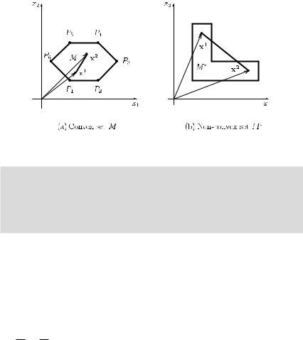
Definition 8.11 A set M is called convex if for any two vectors x1, x2 M , any
convex combination λx1 + (1 − λ)x2 with 0 ≤ λ ≤ 1 also belongs to set M .
310 Linear equations and inequalities
The definition of a convex set is illustrated in Figure 8.1. In Figure 8.1(a), set M is convex since every point of the connecting straight line between the terminal points of vectors x1 and x2 also belongs to set M (for arbitrary vectors x1 and x2 ending in M ). However, set M in Figure 8.1(b) is not convex, since for the chosen vectors x1 and x2 not every point on the connecting straight line between the terminal points of both vectors belongs to set M .
Figure 8.1 A convex set and a non-convex set.
Definition 8.12 A vector (point) x M is called the extreme point (or corner point or vertex) of the convex set M if x cannot be written as a proper convex combination of two other vectors of M , i.e. x cannot be written as
x = λx1 + (1 − λ)x2 with x1, x2 M and 0 < λ < 1.
Returning to Figure 8.1, set M in part (a) has six extreme points x(1), x(2), . . . , x(6) or equivalently the terminal points P1, P2, . . . , P6 of the corresponding vectors (here and in the following chapter, we always give the corresponding points Pi in the figures).
In the case of two variables, we can give the following geometric interpretation of a system
of linear inequalities. Assume that the constraints are given as inequalities. The constraints ai1x1 + ai2x2 Ri bi , Ri {≤, ≥}, i = 1, 2, . . . , m, are half-planes which are bounded by the lines ai1x1 + ai2x2 = bi . The ith constraint can also be written in the form
x1 + x2 = 1, si1 si2
where si1 = bi /ai1 and si2 = bi /ai2 are the intercepts of the line with the x1 axis and the x2 axis, respectively (see Figure 8.2).
The non-negativity constraints x1 ≥ 0 and x2 ≥ 0 represent the non-negative quadrant in the two-dimensional space. Thus, when considering a system of m inequalities with two non-negative variables, the feasible region is described by the intersection of m half-planes

Linear equations and inequalities 311
Figure 8.2 Representation of a line by x1 and x2 intercepts.
Figure 8.3 The set of solutions as the intersection of half-planes.
with the non-negative quadrant. This is illustrated for the case m = 3 in Figure 8.3, where the feasible region M is dashed. In Figure 8.3 and figures which follow we use arrows to indicate which of the resulting half-planes of each constraint satisfies the corresponding inequality constraint. The arrows at the coordinate axes indicate that both variables have to be non-negative.
In general, we can formulate the following property.
THEOREM 8.10 The feasible region M of system (8.13) is either empty or a convex set with at most a finite number of extreme points.
PROOF We only prove that, if M = , it is a convex set. Let x1, x2 M , i.e. we have
Ax1 R b, x1 ≥ 0 and Ax2 R b, x2 ≥ 0,
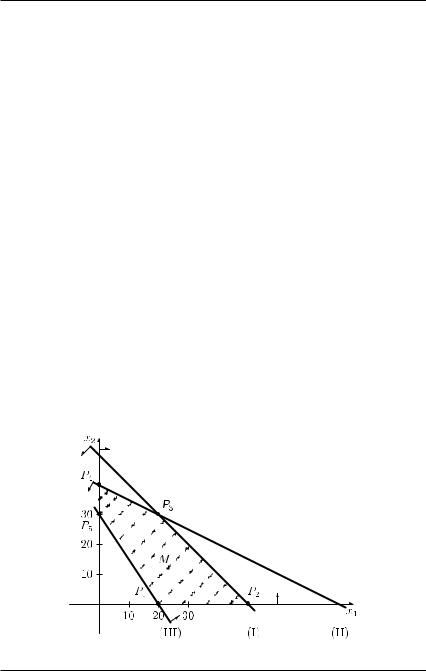

314 Linear equations and inequalities
If the feasible region M is unbounded, there exist (unbounded) one-dimensional rays emanating from some extreme point of M on which points are feasible. Assume that there are u such rays and let r1, r2, . . . , ru denote those vectors pointing from a corresponding extreme point in the direction of such an unbounded one-dimensional ray. Then the feasible region M can be described as follows.
THEOREM 8.12 Let the feasible region M of system (8.13) be unbounded. Then it can be written as follows:
|
s |
|
|
u |
|
|
|
|
|
|
|
|
|
||||
M =*x Rn | x = i |
= |
1 |
λi xi + j |
= |
1 µj rj ; |
|||
|
|
|
|
|
|
|
s |
|
|
|
|
|
|
|
|
||
0 ≤ λi ≤ 1, i = 1, 2, . . . , s, |
i |
= |
1 λi = 1; µ1, µ2, . . . , µu ≥ 0+, |
|||||
|
|
|
|
|
|
|
|
|
where x1, x2, . . . , xs are the extreme points of set M and r1, r2, . . . , ru are the vectors of the unbounded one-dimensional rays of set M .
According to Theorem 8.12, any feasible solution of an unbounded feasible region M can be written as a convex combination of the extreme points and a linear combination of the vectors of the unbounded rays with non-negative scalars µj , j = 1, 2, . . . , u. Considering the example given in Figure 8.4, there are two unbounded one-dimensional rays emanating from points P2 and P3.
A relationship between extreme points and basic feasible solutions is given in the following theorem.
THEOREM 8.13 Any extreme point of the feasible region M of system (8.13) corresponds to at least one basic feasible solution, and conversely, any basic feasible solution corresponds exactly to one extreme point.
The latter theorem needs to be discussed in a bit more detail. We know from our previous considerations that in a basic solution, all non-basic variables are equal to zero. Thus, if the coefficient matrix A of the system of linear equations has rank m, at most m variables have positive values. We can distinguish the following two cases.
Definition 8.13 Let M be the feasible region of system (8.13) and let r(A) = m. If a basic feasible solution x M has m positive components, the solution is called
non-degenerate. If the basic feasible solution x has less than m positive components, the solution is called degenerate.
As we discuss later in connection with linear programming problems in Chapter 9, degeneracy of solutions may cause computational problems. In the case where all basic feasible solutions are non-degenerate solutions, Theorem 8.13 can be strengthened.

Linear equations and inequalities 315
THEOREM 8.14 Let all basic feasible solutions of system (8.13) be non-degenerate solutions. Then there is a one-to-one correspondence between basic feasible solutions and extreme points of the set M of feasible solutions of system (8.13).
8.2.3 A solution procedure
According to Theorem 8.11 we have to generate all extreme points in order to describe the feasible region of a system of linear inequalities. Using Theorems 8.13 and 8.14, respectively, this can be done by generating all basic feasible solutions of the given system.
In this section, we restrict ourselves to the case when system (8.13) is given in the special form
Ax ≤ b, x ≥ 0, with b ≥ 0, |
(8.16) |
where A is an m × n matrix and we assume that r(A) = m. (The case of arbitrary constraints is discussed in detail in the next chapter when dealing with linear programming problems.) This particular situation often occurs in economic applications. For instance, it is necessary to determine feasible production programmes of n goods by means of m raw materials, where the coefficient matrix A describes the use of the particular raw materials per unit of each good and the non-negative vector b describes the capacity constraints on the use of the raw materials.
For a system (8.16), inequalities are transformed into equations by introducing a slack variable in each constraint, i.e. for the ith constraint
ai1x1 + ai2x2 + · · · + ainxn ≤ bi ,
we write
ai1x1 + ai2x2 + · · · + ainxn + ui = bi,
where ui ≥ 0 is a so-called slack variable (i {1, 2, . . . , m}). In the following, we use the m-dimensional vector u = (u1, u2, . . . , um)T for the slack variables introduced in the given m inequalities.
Letting
A = (A, I ) and |
|
= |
x |
, |
x |
u |
the system turns into
A x = b with x = |
x |
≥ 0. |
(8.17) |
u |
In this case, we can choose
x = |
u |
= |
b |
|
x |
|
0 |
as an initial basic feasible solution, i.e. the variables x1, x2, . . . , xn are the non-basic variables and the slack variables u1, u2, . . . , um are the basic variables. Moreover, we assume that x is a non-degenerate basic feasible solution (which means that b > 0).

316 Linear equations and inequalities
Starting with this basic feasible solution, we systematically have to generate all other basic feasible solutions. To this end, we have to determine the pivot element in each step such that the new basic solution is again feasible. (Such pivoting steps are repeated until all basic feasible solutions have been visited.)
|
|
|
|
× |
|
= |
|
|
|
|
+m |
|
|
|
For an m |
|
n matrix A with r(A) |
|
m, there are at most |
n+m |
different basic feasi- |
||||||||
ble solutions of system (8.17) and therefore at most |
|
n |
m |
|
extreme points x of the set |
|||||||||
M |
= { |
x |
|
Rn |
|
|
corresponds to a move from an extreme point |
|||||||
|
|
|
+ | Ax ≤ b}. Each pivoting step |
|
|
|
|
|
|
|
||||
(represented by some basic feasible solution) to another basic feasible solution (usually corresponding to another extreme point). We can use the tableau in Table 8.2 to perform a pivoting step. Rows 1 to m represent the initial basic feasible solution, and rows m + 1 to 2m represent the basic solution obtained after the pivoting step. (As before, we could also add an additional column to describe the operations that have to be performed in order to get rows m + 1 to 2m.)
Table 8.2 Tableau for a pivoting step
Row |
bv |
x1 |
|
· · · |
xl |
· · · |
xn |
|
u1 . . . |
uk |
. . . um |
b |
|
|||||
1 |
u1 |
a11 |
|
· · · |
a1l |
· · · |
a1n |
|
1 . . . |
0 |
|
. . . |
0 |
|
b1 |
|
||
. |
. |
. |
|
|
. |
|
. |
|
. |
. |
|
|
. |
. |
|
|
||
. |
. |
. |
|
|
. |
|
. |
|
. |
. |
|
|
. |
. |
|
|
||
. |
. |
. |
|
· · · |
. |
· · · |
. |
|
. |
. |
|
|
. |
. |
|
|
||
k |
uk |
ak1 |
|
akl |
akn |
|
0 . . . |
1 |
|
. . . |
0 |
bk |
|
|||||
. |
. |
. |
|
|
. |
|
. |
|
. |
. |
|
|
. |
. |
|
|
||
. |
. |
. |
|
|
. |
|
. |
|
. |
. |
|
|
. |
. |
|
|
||
. |
. |
. |
|
· · · |
. |
· · · |
. |
|
. |
. |
|
|
. |
. |
|
|
||
m |
um |
am1 |
|
aml |
amn |
|
0 . . . |
0 |
|
. . . |
1 |
bm |
|
|||||
m + 1 u1 |
a1l |
ak1 |
· · · 0 · · · |
a1l |
akn |
1 . . . |
|
a1l |
|
|
|
a1l |
bk |
|||||
a11 − akl |
a1n − akl |
− akl |
. . . |
0 b1 − akl |
||||||||||||||
. |
. |
. |
|
|
. |
|
. |
|
. |
. |
|
|
. |
. |
|
|
||
. |
. |
. |
|
|
. |
|
. |
|
. |
. |
|
|
. |
. |
|
|
||
. |
. |
. |
|
|
. |
|
. |
|
. |
. |
|
|
. |
. |
|
|
||
m + k xl |
ak1 |
|
· · · |
1 · · · |
akn |
|
0 . . . |
1 |
|
. . . |
0 |
|
bk |
|
||||
akl |
|
akl |
|
|
akl |
|
|
akl |
|
|
||||||||
. |
. |
. |
|
|
. |
|
. |
|
. |
. |
|
|
. |
. |
|
|
||
. |
. |
. |
|
|
. |
|
. |
|
. |
. |
|
|
. |
. |
|
|
||
. |
. |
. |
|
|
. |
|
. |
|
. |
. |
|
|
. |
. |
|
|
||
2m um |
aml |
ak1 |
· · · |
0 · · · |
aml |
akn |
0 . . . |
|
aml |
|
|
|
aml |
bk |
||||
am1 − akl |
amn − akl |
− akl |
. . . |
1 bm − akl |
||||||||||||||
Assume that we choose akl = 0 as pivot element, i.e. we replace the basic variable uk by the original non-basic variable xl . Then we obtain the new basic solution
|
= |
x |
|
x |
|
||
u |
|||
with
|
|
|
|
|
|
|
|
|
|
|
|
|
bk |
|
|
|
|
|
xT = (x1, . . . , xl , . . . , xn) = |
0, . . . , |
, . . . , 0 |
|
|
||||||||||||
|
|
akl |
|
|
|||||||||||||
and |
|
|
|
|
|
|
|
||||||||||
|
|
|
|
|
|
|
|
|
|
|
|
a1l |
aml |
· bk . |
|||
|
uT = (u1, . . . , uk , . . . , um) = b1 − |
|
|
· bk , . . . , 0, . . . , bm − |
|
||||||||||||
|
akl |
akl |
|||||||||||||||
The new basic solution
|
= |
x |
|
x |
|
||
u |
|||

Linear equations and inequalities 317
is feasible if all components of vector x are non-negative, i.e.
|
bk |
≥ 0 |
(8.18) |
||
|
akl |
||||
and |
|
|
|
|
|
bi − |
ail |
· bk ≥ 0, i = 1, 2, . . . , m, i = k. |
(8.19) |
||
akl |
|||||
Next, we derive a condition such that both (8.18) and (8.19) are satisfied. First, since b > 0 (remember that we are considering a non-degenerate solution) and akl = 0 by assumption, we have the equivalence
bk |
≥ 0 |
akl > 0. |
akl |
This means that in the chosen pivot column, only positive elements are a candidate for the pivot element. However, we also have to ensure that (8.19) is satisfied. We get the following equivalence:
bi − |
ail |
· bk ≥ 0 |
|
bi |
≥ |
bk |
≥ 0 for all i with ail > 0. |
akl |
ail |
akl |
This means that we have to take that row as pivot row, which yields the smallest quotient of the current right-hand side component and the corresponding element in the chosen pivot column among all rows with a positive element in the pivot column. Summarizing, we can replace the basic variable uk by the non-basic variable xl if
|
|
|
bk |
|
bi |
|
|
|
|
|
|
|
|
akl > 0 |
and |
qk = |
akl |
= min |
ail |
ail > 0, i {1, 2, . . . , m} . |
If one of the above conditions is violated, i.e. if akl < 0 or quotient qk = bk /akl is not minimal among all quotients in the rows with a positive element in the pivot column, we do not get a basic feasible solution, i.e. at least one component of the new right-hand side vector would be negative. Therefore, we add a column Q in the tableau in Table 8.2 to calculate the corresponding quotients qi which have to be taken into account. Notice that in the new tableau, there is again an identity submatrix (with possibly interchanged columns) contained in the transformed matrix belonging to the basic variables.
In the case of a degenerate basic feasible solution, all the above formulas for a pivoting step remain valid. In such a case, we have a smallest quotient qk = 0 (which, by the way, means that also in the case of choosing a negative pivot element a basic feasible solution results). We will discuss the difficulties that may arise in case of degeneracy later in Chapter 9 in a bit more detail.
The process of enumerating all basic feasible solutions of system (8.13) can be done by hand (without using a computer) only for very small problems. Consider the following example.
Example 8.12 Consider the system of linear inequalities presented in Example 8.10. Introducing slack variables u1, u2 and u3, we obtain the initial tableau in rows 1 to 3 below. Now, the goal is to generate all basic feasible solutions of the given system of linear equations.

318 Linear equations and inequalities
Since each basic feasible solution has three basic variables, there are at most 53 = 10 basic feasible solutions. We successively perform pivoting steps and might obtain for instance the following sequence of basic feasible solutions:
Row |
bv |
x1 |
x2 |
u1 |
|
u2 |
|
u3 |
b |
Q |
1 |
u1 |
−2 |
1 |
|
1 |
|
0 |
0 |
0 |
− |
2 |
u2 |
1 |
−1 |
|
0 |
|
1 |
0 |
4 |
4 |
3 |
u3 |
1 |
1 |
|
0 |
|
0 |
1 |
30 |
30 |
4 |
u1 |
0 |
−1 |
|
1 |
|
2 |
0 |
8 |
− |
5 |
x1 |
1 |
−1 |
|
0 |
|
1 |
0 |
4 |
− |
6 |
u3 |
0 |
2 |
|
0 |
−1 |
1 |
26 |
13 |
|
7 |
u1 |
0 |
0 |
|
1 |
|
3 |
1 |
21 |
14 |
|
|
2 |
2 |
|||||||
8 |
x1 |
1 |
0 |
|
0 |
|
1 |
1 |
17 |
34 |
|
|
2 |
2 |
|||||||
9 |
x2 |
0 |
1 |
|
0 |
− |
1 |
1 |
13 |
− |
|
2 |
2 |
||||||||
10 |
u2 |
0 |
0 |
|
2 |
|
1 |
1 |
14 |
42 |
|
3 |
|
3 |
|||||||
11 |
x1 |
1 |
0 |
− |
1 |
|
0 |
1 |
10 |
30 |
3 |
|
3 |
||||||||
12 |
x2 |
0 |
1 |
|
1 |
|
0 |
2 |
20 |
30 |
|
3 |
|
3 |
|||||||
The corresponding pivot elements are printed in bold face. In the first tableau (rows 1 to 3), we can choose either the column belonging to x1 or that belonging to x2 as pivot column (since there is at least one positive element in each of these columns). Selecting the column belonging to x1, the quotient is uniquely determined, and we have to replace the basic variable u2 by the non-basic variable x1. In the second pivoting step, we can choose only the column belonging to x2 as pivot column (since, when choosing the column belonging to u2, we come back to the basic feasible solution represented by rows 1 to 3).
From the last basic feasible solution, we cannot generate another extreme point. However, we can perform another pivoting step so that u3 becomes a basic variable. Determining now the minimum quotient in the Q column, it is not uniquely determined: we can choose x1 or x2 as the variable that becomes a non-basic variable (since in both cases, we have the smallest quotient 30). If we choose x1 as the variable that becomes a non-basic variable, we get the tableau:
Row |
bv |
x1 |
x2 |
u1 |
u2 |
u3 |
b Q |
13 |
u2 |
−1 |
0 |
1 |
1 |
0 |
4 |
14 |
u3 |
3 |
0 |
−1 |
0 |
1 |
30 |
15 |
x2 |
−2 |
1 |
1 |
0 |
0 |
0 |
If we choose in the fourth tableau x2 as the variable that becomes a non-basic variable, we get the following tableau:
Row |
bv |
x1 |
x2 |
|
u1 |
u2 |
u3 |
b Q |
16 |
u2 |
0 |
− |
1 |
1 |
1 |
0 |
4 |
2 |
2 |
|||||||
17 |
x1 |
1 |
− 21 |
− 21 |
0 |
1 |
0 |
|
18 |
u3 |
0 |
|
3 |
1 |
0 |
1 |
30 |
|
2 |
2 |
||||||
|
|
|
|
|
|
|
|
|
|
|
|
|
|
|
|
|
|
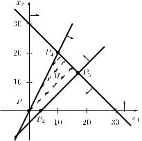

320 Linear equations and inequalities
have been visited and the procedure stops. According to Theorem 8.10, the feasible region is given by the set of all convex combinations of the four extreme points:
M = x2 |
R2 |
|
|
x2 |
|
= λ1 0 + λ2 0 + λ3 13 + λ4 20 ; |
|||
x1 |
|
|
|
x1 |
|
0 |
4 |
17 |
10 |
|
|
|
|
|
|
4 |
|
|
|
|
|
|
|
|
|
|
|
|
|
λi ≥ 0, i {1, 2, 3, 4}, |
λi = 16 . |
|
|
|
|||||
i=1
Since the columns belonging to the basic variables are always unit vectors, they can be omitted. All required information for performing a pivoting step is contained in the columns of the non-basic variables. Therefore, we can use a short form of the tableau, where the columns are assigned to the non-basic variables and the rows are assigned to the basic variables. Assume that altogether n variables denoted by x1, x2, . . . , xn occur in the system of linear inequalities; among them there are m basic variables denoted by xB1, xB2, . . . , xBm and n = n − m non-basic variables denoted by xN 1, xN 2, . . . , xNn . In this case, the short form of the tableau is as in Table 8.3.
Table 8.3 Short form of the tableau for a pivoting step
Row |
bv |
|
xN 1 |
|
· · · |
xNl |
· · · |
xN n |
|
|
|
|
|
|
|
|
|
|||||||||||||||||
|
1 |
|
xB1 |
|
a |
|
· · · |
|
a |
· · · |
a |
|
|
|
|
|
|
b |
|
|
||||||||||||||
|
|
|
|
|
|
11 |
|
|
|
|
|
1l |
|
1n |
|
|
|
1 |
|
|
|
|||||||||||||
|
. |
. |
|
. |
|
|
|
|
. |
|
|
|
. |
|
|
|
|
|
|
. |
|
|
|
|||||||||||
|
. |
. |
|
. |
|
|
|
|
. |
|
|
|
. |
|
|
|
|
|
|
. |
|
|
|
|||||||||||
|
. |
. |
|
. |
|
|
|
· · · |
. |
|
· · · |
. |
|
|
|
|
|
|
. |
|
|
|
||||||||||||
|
|
|
xBk |
|
|
k1 |
|
|
|
|
kl |
|
kn |
|
|
|
|
k |
|
|
||||||||||||||
|
k |
|
|
a |
|
|
|
a |
|
|
a |
|
|
|
b |
|
|
|||||||||||||||||
|
. |
. |
|
. |
|
|
|
|
. |
|
|
|
. |
|
|
|
|
|
|
. |
|
|
|
|||||||||||
|
. |
. |
|
. |
|
|
|
|
. |
|
|
|
. |
|
|
|
|
|
|
. |
|
|
|
|||||||||||
|
. |
. |
|
. |
|
|
|
· · · |
. |
|
· · · |
. |
|
|
|
|
|
|
. |
|
|
|
||||||||||||
|
|
xBm |
|
|
m1 |
|
|
|
ml |
|
mn |
|
|
|
|
m |
|
|
||||||||||||||||
|
m |
|
a |
|
|
a |
|
|
a |
|
|
|
|
|
|
b |
|
|
||||||||||||||||
|
|
|
|
|
|
xN 1 |
|
. . . |
|
|
|
Nl |
. . . |
xN n |
|
|
|
|
|
|
|
|
|
|||||||||||
|
|
|
|
|
|
|
x |
|
|
|
|
|
|
|
|
|
||||||||||||||||||
|
|
|
|
|
a |
|
|
a |
a |
|
|
|
|
a |
|
|
a |
a |
a |
b |
|
|
a |
b |
||||||||||
m |
|
1 xB1 |
|
|
1l |
|
|
|
|
|
|
1l |
. . . |
|
1l |
|
|
|
1l |
|||||||||||||||
+ |
− akl |
· · · − akl |
|
|
|
− akl |
||||||||||||||||||||||||||||
|
. |
11 |
k1 |
|
|
1n − akl |
|
kn |
1 |
|
k |
|||||||||||||||||||||||
|
. |
|
. |
|
|
|
|
. |
|
|
|
. |
|
|
|
|
|
|
. |
|
|
|
||||||||||||
|
. |
. |
|
. |
|
|
|
|
. |
|
|
|
. |
|
|
|
|
|
|
. |
|
|
|
|||||||||||
|
. |
. |
|
. |
|
|
|
|
. |
|
|
|
. |
|
|
|
|
|
|
. |
|
|
|
|||||||||||
|
|
|
|
|
|
|
a |
|
|
1 |
|
|
|
|
a |
|
|
|
|
|
|
|
b |
|
|
|||||||||
m + k xBk |
|
|
k1 |
|
· · · |
|
· · · |
|
kn |
|
|
|
|
k |
|
|
||||||||||||||||||
|
|
akl |
|
|
|
|
akl |
|
|
akl |
|
|
|
|
|
akl |
|
|
|
|||||||||||||||
|
. |
. |
|
. |
|
|
|
|
. |
|
|
|
. |
|
|
|
|
|
|
. |
|
|
|
|||||||||||
|
. |
. |
|
. |
|
|
|
|
. |
|
|
|
. |
|
|
|
|
|
|
. |
|
|
|
|||||||||||
|
. |
. |
|
. |
|
|
|
|
. |
|
|
|
. |
|
|
|
|
|
|
. |
|
|
|
|||||||||||
|
|
|
|
|
a |
|
|
a |
a |
|
|
|
|
a |
|
|
a |
a |
|
a |
b |
|
|
a |
|
b |
||||||||
2m |
xBm |
|
|
ml |
|
|
|
|
|
ml |
|
|
|
ml |
|
|
|
ml |
||||||||||||||||
|
|
|
· · · − akl |
· · · |
|
|
|
|
|
|||||||||||||||||||||||||
|
|
|
|
|
m1 |
− akl |
k1 |
mn − |
|
akl |
|
kn |
m |
− akl |
|
k |
||||||||||||||||||
In column bv, the basic variables xB1, xB2, . . . , xBm are given, and the next n columns represent the non-basic variables xN 1, xN 2, . . . , xNn . After the first pivoting step, the kth basic variable is now the former lth non-basic variable: xBk = xNl . Correspondingly, the lth nonbasic variable in the new solution is the former kth basic variable: xNl = xBk . Notice that in each transformation step we have to write the sequence of the non-basic variables since the variables in the columns do not appear according to the numbering.

Linear equations and inequalities 321
It is worth emphasizing that, in contrast to the full form of the tableau, the new elements ail of the pivot column are obtained as follows:
1
akl = , akl
a
a = − il , i = 1, 2, . . . , m, i = k,
il akl
i.e. the pivot element is replaced by its reciprocal value and the remaining elements of the pivot column are divided by the negative pivot element. Notice that this column also occurs in the full form of the tableau, though not in the pivot column (where after the pivoting step a unit vector occurs) but it appears in the column of the new non-basic variable xNl in the full form of the tableau after the pivoting step. The following example uses the short form of this tableau.
Example 8.13 We consider the following system of linear inequalities:
|
+ |
x2 |
≤ |
25 |
2x1 |
x2 |
≤ |
30 |
|
−x1 |
+ |
x2 |
≥ |
−6 |
|
|
x1, x2 |
≥ |
0. |
We multiply the third constraint by −1 and introduce in each inequality a slack variable denoted by u1, u2 and u3. This yields a system with three equations and five variables.
|
+ |
x2 |
+ u1 |
= 25 |
2x1 |
x2 |
+ u2 |
= 30 |
|
x1 |
− |
x2 |
|
+ u3 = 6 |
x1, x2, u1, u2, u3 ≥ 0.
There are at most = 10 basic feasible solutions, each of them including exactly three basic variables. In order to describe the feasible region, we have to generate systematically all the possible basic feasible solutions. Starting from the first basic solution with x1 = 0, x2 = 0, u1 = 25, u2 = 30, u3 = 6 and using the short form of the tableau, we obtain e.g. the following sequence of basic feasible solutions by subsequent pivoting steps. In the first step we have chosen the column belonging to x1 as pivot column. (This is possible since at least one element in this column is positive; analogously one can also start with the column belonging to x2 as the first pivot column.) Using the quotients in the Q column, we have found that row 3 must be the pivot row and, therefore, we have the pivot element 1. From the tableau given by rows 4 to 6, we have to select the column belonging to variable x2 as pivot column (otherwise we come back to the basic feasible solution described by rows 1 to 3). The quotient rule determines row 5 as pivot row. Continuing in this way (note that the pivot column is now always uniquely determined since in the other case we would always go back to the previous basic feasible solution), we get the results in the following tableaus.
322 Linear equations and inequalities
Row |
bv |
x1 |
x2 |
|
b |
Q |
1 |
u1 |
0 |
|
1 |
25 |
− |
2 |
u2 |
2 |
|
1 |
30 |
15 |
3 |
u3 |
1 |
−1 |
6 |
6 |
|
|
|
u3 |
x2 |
|
|
|
4 |
u1 |
0 |
|
1 |
25 |
25 |
5 |
u2 |
−2 |
|
3 |
18 |
6 |
6 |
x1 |
1 |
−1 |
6 |
− |
|
|
|
u3 |
u2 |
|
|
|
7 |
u1 |
2 |
− |
1 |
19 |
57 |
3 |
3 |
2 |
||||
8 |
x2 |
2 |
|
1 |
6 |
− |
− 3 |
|
3 |
||||
9 |
x1 |
1 |
|
1 |
12 |
36 |
3 |
|
3 |
||||
|
|
u1 |
u2 |
|
|
|
10 |
u3 |
3 |
− |
1 |
57 |
− |
2 |
2 |
2 |
||||
11 |
x2 |
1 |
|
0 |
25 |
− |
12 |
x1 |
1 |
|
1 |
5 |
5 |
− 2 |
|
2 |
2 |
|||
|
|
u1 |
x1 |
|
|
|
13 |
u3 |
− 21 |
|
1 |
31 |
|
14 |
x2 |
1 |
|
0 |
25 |
|
15 |
u2 |
−1 |
|
2 |
5 |
|
Having generated the above five basic feasible solutions, we can stop our computations for the following reasons. There remain five other selections of three variables out of the variables x1, x2, u1, u2, u3 which, however, do not yield basic feasible solutions. The variables x2, u1, u3 as basic variables lead to a basic infeasible solution. (When selecting x2 as the variable that becomes a basic variable in the next solution and row 2 as pivot row, this would violate the quotient rule since q2 = 30 > q1 = 25.) Similarly, the choice of x1, u1, u3 as basic variables does not lead to a basic feasible solution since we would violate the quotient rule when choosing the x1 column as pivot column and row 2 as pivot row. The choice of x1, u2, u3 as basic variables is not possible because when choosing the x1 column as pivot column and row 1 as pivot row in the first tableau, pivot zero would result and this is not allowed (i.e. the corresponding column vectors of matrix A belonging to these variables are linearly dependent). The choice of x1, x2, u2 as basic variables leads to a basic infeasible solution because when choosing the u2 column as pivot column and row 7 as pivot row in the third tableau, the resulting pivot element would be negative. For the same reason, the choice of variables x2, u1, u2 as basic variables does not lead to a basic feasible solution. (Selecting the x2 column as pivot column and row 3 as pivot row in the first tableau yields the negative pivot −1.) Therefore, in addition to the five basic feasible solutions determined from rows 1 to 15, there are four further basic infeasible solutions.
From the above five basic feasible solutions, we obtain the resulting five extreme points of the feasible region M (by dropping the slack variables u1, u2 and u3). Therefore, set M is

|
|
|
|
|
|
|
|
Linear equations and inequalities 323 |
|||||
given by |
R+ |
|
|
|
|
= λ1 0 + λ2 0 + λ3 |
|
|
|||||
M = x2 |
x2 |
6 |
|||||||||||
x1 |
|
2 |
|
|
x1 |
|
0 |
6 |
|
|
|
12 |
|
|
|
|
|
|
|
|
|
||||||
|
|
|
|
|
|
|
|
|
5 |
|
|
|
|
|
5/2 |
|
|
|
|
0 |
|
|
|
|
|
||
+λ4 |
25 |
+ λ5 25 |
; λi ≥ 0, i = 1, 2, . . . , 5, |
i |
= |
1 λi = 16 . |
|||||||
|
|
|
|
|
|
|
|
|
|
|
|
|
|
The graphical solution of the system of linear inequalities is given in Figure 8.7. The ith basic feasible solution corresponds to extreme point Pi . In this example, there is exactly one basic feasible solution corresponding to each extreme point since each basic feasible solution is non-degenerate.
Figure 8.7 Feasible region for Example 8.13.
EXERCISES
8.1Decide whether the following systems of linear equations are consistent and find the solutions. Apply both methods of Gaussian elimination and pivoting (use the rank criterion).
(a) x1 |
+ 2x2 |
+ 3x3 |
= 5 |
2x1 |
+ 3x2 |
+ x3 |
= 8 |
3x1 |
+ x2 |
+ 2x3 |
= 5 |
(b) 3x1 |
+ x2 |
+ x3 |
= 3 |
4x1 |
− x2 |
+ 2x3 |
= 4 |
x1 |
− x2 |
+ x3 |
= 1 |
4x1 |
− x2 |
+ 2x3 |
= 5 |
324 Linear equations and inequalities
(c) 3x1 |
+ 4x2 |
+ x3 |
+ 6x4 |
= 8 |
3x1 |
+ 8x2 |
+ 6x3 |
+ 5x4 |
= 7 |
8x1 |
+ 5x2 |
+ 6x3 |
+ 7x4 |
= 6 |
6x1 |
+ 2x2 |
+ 5x3 |
+ 3x4 |
= 5 |
(d) x1 |
+ 2x2 |
+ 3x3 |
= 16 |
|
8x1 |
+ 7x2 |
+ 6x3 |
= 74 |
|
4x1 |
+ 5x2 |
+ 9x3 |
= 49 |
|
5x1 |
+ 4x2 |
+ 2x3 |
= 43 |
|
x1 |
+ 4x2 |
+ x3 |
= 22. |
|
8.2(a) Solve the following homogeneous systems of linear equations Ax = 0 with
|
= |
|
1 |
1 |
1 |
1 |
|
|
= |
|
1 |
1 |
1 |
1 |
|
(i) A |
2 3 |
5 |
0 |
(ii) A |
2 3 5 |
0 |
|||||||||
|
0 |
1 |
3 |
0 |
; |
|
2 |
3 |
6 |
3 |
|
||||
|
|
|
|
|
|
|
|
|
|
|
|
|
|
|
|
|
|
|
1 |
1 |
2 |
4 |
|
|
|
|
1 |
1 |
2 |
4 |
|
|
|
|
|
|
|
|
|
||||||||
(b)Find the solutions of the non-homogeneous system Ax = b with matrix A from
(i) resp. (ii) and b = (0, 0, −2, 2)T.
8.3Find the general solutions of the following systems and specify two different basic solutions for each system:
(a) 4x1 |
− x2 |
− 3x3 |
+ 5x4 |
= −2 |
||||
−x1 |
+ |
x2 |
+ |
x3 |
− |
x4 |
= |
4 |
2x1 |
− |
x2 |
− |
x3 |
− |
2x4 |
= |
1 |
(b) x1 |
+ 2x2 |
− x3 |
+ |
|
+ 4x5 |
= 2 |
||||
x1 |
+ 4x2 |
− 5x3 |
x4 |
+ 3x5 |
= 1 |
|||||
2x1 |
− |
2x2 |
+ |
10x3 |
+ |
x4 |
− |
x5 |
= |
11 |
3x1 |
+ |
2x2 |
+ |
5x3 |
+ 2x4 |
+ |
2x5 |
= |
12 |
|
8.4What restriction on the parameter a ensures the consistence of the following system? Find the solution depending on a.
3x |
+ |
4y |
+ |
4z |
= |
2 |
3x |
+ |
2y |
+ |
3z |
= |
3 |
4x |
+ |
5y |
+ |
az |
= |
4 |
8.5Check the consistence of the following system as a function of the parameter λ:
3x |
+ |
2y |
+ |
z |
= |
0 |
6x |
+ |
4y |
+ |
λz |
= |
0 |
Do the following cases exist?
(a)There is no solution.
(b)There is a unique solution.
Find the solution if possible.
Linear equations and inequalities 325
8.6Given is the system
0 1 −1 |
−1 |
x2 |
3 . |
||||||||
|
1 |
0 |
0 |
1 |
|
x1 |
|
|
|
2 |
|
0 1 |
0 |
b |
x3 |
|
= |
0 |
|
||||
|
|
|
|
|
|
4 |
|
|
|
|
|
|
0 |
0 |
a |
0 |
|
x |
|
|
|
1 |
|
|
|
|
|
|
|
||||||
(a)Decide with respect to the parameters a and b in which cases the system is consistent or inconsistent. When does a unique solution exist?
(b)Find the general solution if possible.
(c)Calculate the solution for a = 1 and b = 0.
8.7Decide whether the following system of linear equations is consistent and find the solution in dependence on parameters a and b:
a x + (a + b) y + b z = 3a + 5b
b x |
+ |
ab y |
+ |
a z |
= |
a(2b + 3) + b |
a x |
+ |
b y |
+ |
b z |
= |
a + 5b |
8.8Find the kernel of the linear mapping described by matrix
A |
5 |
−1 |
7 |
. |
|
2 |
−2 |
2 |
|
|
= 3 |
−1 |
4 |
8.9Given are the two systems of linear equations
x1 |
+ 2x2 |
+ 3x3 |
= 5 |
x1 |
+ 2x2 |
+ 3x3 |
= 14 |
||||||
3x1 |
+ |
1x2 |
+ |
2x3 |
= |
5 |
and 2x1 |
+ |
3x2 |
+ |
x3 |
= |
13 |
2x1 |
+ |
3x2 |
+ |
1x3 |
= |
8 |
3x1 |
+ |
x2 |
+ |
2x3 |
= |
21. |
Solve them in only one tableau.
8.10Find the inverse matrices by pivoting:
|
|
|
− |
1 |
3 |
2 |
|
2 |
1 |
4 |
6 |
|
(a) |
|
|
1 |
− 0 |
− 1 |
|
2 |
1 |
||||
A = |
2 |
5 |
3 |
; |
|
(b) B = 3 |
; |
|||||
|
|
|
|
3 |
8 |
4 |
|
|
7 |
8 |
8 |
|
(c) |
C |
= |
−1 |
2 |
− |
−4 |
|
|
|
|
||
2 |
|
|
|
|||||||||
|
|
2 |
−1 |
−2 |
|
3 |
. |
|
|
|
||
|
|
|
|
|
|
|
|
|
|
|
|
|
|
|
|
|
|
|
|
|
|
|
|
|
|
01 2 −5
8.11Find the solutions of the following matrix equations:
(a)XA = B with
|
= |
|
3 |
|
8 |
|
4 |
|
= |
|
− |
|
|
|
|
|
1 |
|
3 |
|
2 |
|
1 |
4 |
|
2 |
|
A |
|
− |
|
− |
5 |
− |
3 |
|
and B 3 |
−3 |
|
2 |
; |
|
−2 |
|
|
|
|
||||||||
326Linear equations and inequalities
(b)AXB = C with
A = |
−1 |
2 |
, |
|
B = |
4 |
3 |
|
|
and |
|
C = |
1 |
0 |
; |
||
|
|
2 |
1 |
|
|
|
3 |
2 |
|
|
|
|
|
|
0 |
1 |
|
(c) XA = −2(X + B) with |
|
|
|
|
= |
|
|
− |
|
|
|
|
|||||
|
= |
2 |
1 |
|
2 |
|
|
|
|
|
|
|
|
||||
|
|
−3 |
1 |
− |
1 |
|
|
|
|
|
2 |
4 |
|
0 |
|
|
|
A |
|
|
0 |
1 |
and |
|
B |
|
1 |
−3 |
|
2 . |
|
|
|||
|
−1 |
|
|
|
|
|
|
|
|||||||||
8.12Assume we have a four-industry economy. Each industry is to produce an output just sufficient to meet its own input requirements and those of the other three industries as well as the final demand of the open sector. That is, the output level xi must satisfy the following equation:
xi = xi1 + xi2 + xi3 + xi4 + yi, i {1, 2, 3, 4},
where yi is the final demand for industry i and xij is the amount of xi needed as input for the industry j {1, 2, 3, 4}. Let
|
= |
|
= |
|
5 |
15 |
15 |
10 |
|
|
= |
|
5 |
|
X |
(xij ) |
10 |
30 |
15 |
25 |
and y |
20 |
|||||||
|
|
25 |
25 |
10 |
30 |
|
|
10 |
. |
|||||
|
|
|
|
|
|
|
|
|
|
|
|
|
|
|
|
|
|
|
|
10 |
20 |
20 |
20 |
|
|
|
|
30 |
|
|
|
|
|
|
|
|
|
|
|
|||||
(a)Find the input-coefficient matrix A which satisfies the equation x = Ax + y
with x = (x1, x2, x3, x4)T and xij = aij xj . |
y |
= |
||
(b) How does the |
matrix X change if the final demand changes to |
|||
T |
and the input coefficients are constant? |
|
||
(10, 20, 20, 15) |
|
|
|
|
8.13Given is the bounded convex set with the extreme points
x1 |
|
|
2 |
|
x2 |
= |
1 |
|
x3 |
2 |
|
|
x4 |
= |
1 |
|
|
= 0 |
1 |
= 1 |
|
1 |
|||||||||||||
|
1 |
, |
|
1 |
, |
0 |
|
and |
−3 |
. |
|||||||
Do the points |
|
|
|
|
|
|
|
|
|
|
|
|
|
||||
|
|
|
1 |
2 |
|
|
|
|
|
1 |
|
|
|
|
|
|
|
|
= |
1 |
|
|
|
|
|
= 2 |
|
|
|
|
|
|
|
||
a |
|
|
|
3 |
|
and |
|
b |
0 |
|
|
|
|
|
|
|
|
|
|
2 |
|
|
|
|
|
|
|
||||||||
belong to the convex set given above?
8.14In addition to its main production a firm produces two products A and B with two machines I and II. The products are manufactured on machine I and packaged on machine II. Machine I has a free capacity of 40 hours and machine II can be used for 20 hours. To produce 1 tonne of A takes 4 min on machine I and 6 min on machine II.
Linear equations and inequalities 327
Producing 1 tonne of B takes 10 min on machine I and 3 min on machine II. What output combinations are possible?
(a)Model the problem by means of a system of linear inequalities.
(b)Solve the problem graphically.
(c)Find the general solution by calculation.
8.15Solve the following problem graphically:
−x1 |
+ |
x2 |
≤ |
4 |
−2x1 |
+ |
x2 |
≤ |
3 |
x1 |
− |
2x2 |
≤ |
1 |
|
|
x1, x2 |
≥ |
0 |
8.16Find the general solutions of the following systems by calculation:
(a) |
2x1 |
+ |
5x2 |
− 2x3 |
≤ |
5 |
|
4x1 |
+ x2 |
+ x3 |
≤ 3 |
||
|
|
|
|
x1, x2, x3 |
≥ |
0 |
(b) |
x1 |
+ |
x2 + |
x3 |
≤ |
3 |
|
x1 |
|
+ |
5x3 |
≤ |
3 |
|
|
|
|
x1, x2, x3 |
≥ |
0 |