Добавил:

Upload Опубликованный материал нарушает ваши авторские права? Сообщите нам.

Вуз:

Донецкий национальный технический университет

Предмет:

[НЕСОРТИРОВАННОЕ]

Файл:

Mathematics of Economics and Business.pdf

Скачиваний:

Добавлен:

03.03.2016

Размер:

8.37 Mб

Скачать

☆

<<< < Предыдущая 1 2 3 45 / 175 6 7 8 9 10 11 12 13 14 15 16 17 > Следующая >>>

2Sequences; series; finance

This chapter deals first with sequences and series. Sequences play a role e.g. when solving difference equations. Special types of sequences and series are closely related to problems in finance, which we discuss at the end of this chapter.

2.1 SEQUENCES

2.1.1 Basic definitions

Definition 2.1 If to each positive integer n N, there is assigned a real number an, then

{an} = a1, a2, a3, . . . , an, . . .

is called a sequence.

The elements a1, a2, a3, . . . are called the terms of the sequence. In particular an is denoted as the nth term. There are two ways of defining a sequence:

(1)explicitly by giving the nth term of the sequence;

(2)recursively by giving the first term(s) of the sequence and a recursive formula for calculating the remaining terms.

This is illustrated by the following example.

Example 2.1 (a) Consider the sequence {an} with

a	n =		n − 1			,			n		N.
a						,			n		N.
			2n	+	1
				+
We get the terms
a1 =				a2 =			1			a3 =		2		a4 =	3			a5 =	4
		0,						,					,				,			, . . . .
		0,					5	,				7	,			9	,		11	, . . . .

In this case, sequence {an} is given explicitly.

62 Sequences; series; finance

(b) Let sequence {bn} be given by

b1 = 2 and bn+1 = 2bn − 1, n N.

Then we get the terms

b1 = 2, b2 = 3, b3 = 5, b4 = 9, b5 = 17, . . . .

The latter sequence is given recursively.

cn = (−1)n, n N.

In this case, we get the terms

c1 = −1, c2 = 1, c3 = −1, c4 = 1, c5 = −1, . . . .

This is an alternating sequence, where any two successive terms have a different sign.

Arithmetic and geometric sequences

We continue with two special types of sequences.

Definition 2.2 A sequence {an}, where the difference of any two successive terms is constant, is called an arithmetic sequence, i.e.

an+1 − an = d for all n N, where d is constant.

Thus, the terms of an arithmetic sequence with the first term a1 follow the pattern

a1, a1 + d, a1 + 2d, a1 + 3d, . . . , a1 + (n − 1)d, . . .

and we obtain the following explicit formula for the nth term:

an = a1 + (n − 1)d for all n N.

Example 2.2 A car company produces 750 cars of a certain type in the first month of its production and then in each month the production is increased by 20 cars in comparison with the preceding month. What is the production in the twelfth month?

This number is obtained as the term a12 of an arithmetic sequence with a1 = 750 and d = 20, and we get

a12 = a1 + 11 · d = 750 + 11 · 20 = 970,

i.e. in the twelfth month, 970 cars of this type have been produced.

Sequences; series; finance 63

Definition 2.3 A sequence {an}, where the ratio of any two successive terms is the same number q = 0, is called a geometric sequence, i.e.

an+1 = q for all n N, where q is constant. an

Thus, the terms of a geometric sequence with the first term a1 follow the pattern

a1, a1 · q, a1 · q2, a1 · q3, . . . , a1 · qn−1, . . .

and we obtain the following explicit formula for the nth term:

an = a1 · qn−1

for all n N.

Example 2.3 Consider sequence {an} with

an = (−1)n · 4−n,

n N.

The first term is

a1 = (−1)1 · 4−1

= −

Using

an+1 = (−1)n+1 · 4−(n+1)

and

an = (−1)n · 4−n,

we obtain

an+1

(

−

4−n−1+n

= −

4−1

= −

Thus, {an} is a geometric sequence with common ratio q = −1/4.

Example 2.4 A firm produced 20,000 DVD players in its first year 2001. If the production increases every year by 10 per cent, what will be the production in 2009?

The answer is obtained by the ninth term of a sequence {an} with q = 1 + 0.1:

a9 = a1 · q8 = 20, 000 · 1.18 ≈ 42, 872.

Next, we investigate what will be the first year so that under the above assumptions, production will exceed 55,000 DVD players. From

an = 55, 000 = 20, 000 · 1.1n−1 = a1 · qn−1

64 Sequences; series; finance
we obtain
1.1n−1 =	55, 000		= 2.75

	20, 000
and
n − 1 =	ln 2.75		1.0116
			≈		≈ 10.61,
		ln 1.1	≈	0.0953	≈ 10.61,

i.e. n ≈ 11.61. Thus, 2012 will be the first year with a production of more than 55,000 DVD players.

Next, we introduce some basic notions.

Definition 2.4 A sequence {an} is called increasing (resp. strictly increasing) if

an ≤ an+1 (resp. an < an+1)

for all n N.

Sequence {an} is called decreasing (resp. strictly decreasing) if

an ≥ an+1 (resp. an > an+1)

for all n N.

A sequence {an} which is (strictly) increasing or decreasing is also denoted as (strictly) monotone. When checking a sequence {an} for monotonicity, we investigate the difference Dn = an+1 − an of two successive terms. If Dn ≥ 0 (Dn > 0) for all n N, sequence {an} is increasing (strictly increasing). If Dn ≤ 0 (Dn < 0) for all n N, sequence {an} is decreasing (strictly decreasing).

Example 2.5 We investigate sequence {an} with

an = 2(n − 1)2 − n, n N,

for monotonicity, i.e. we investigate the difference of two successive terms and obtain

an+1 − an = 2n2 − (n + 1) − 2(n − 1)2 − n

=2n2 − n − 1 − 2n2 − 4n + 2 − n

=4n − 3.

Since 4n − 3 > 0 for all n N, we get an+1 > an for all n N. Therefore, sequence {an} is strictly increasing.

Sequences; series; finance 65

Definition 2.5 A sequence {an} is called bounded if there exists a finite constant C (denoted as bound) such that

|an| ≤ C

for all n N.

Example 2.6 We consider the sequence {an} with

a	n =	(−1)n · 2	,	n	N,
		n2

and investigate whether it is bounded. We can estimate |an| as follows:

	1)n		2
\|an\| =	(− n2	· 2	= n2	≤ 2 for all n N.

Therefore, sequence {an} is bounded. Note that sequence {an} is not monotone, since the signs of the terms alternate due to factor (−1)n.

2.1.2 Limit of a sequence

Next, we introduce the basic notion of a limit of a sequence.

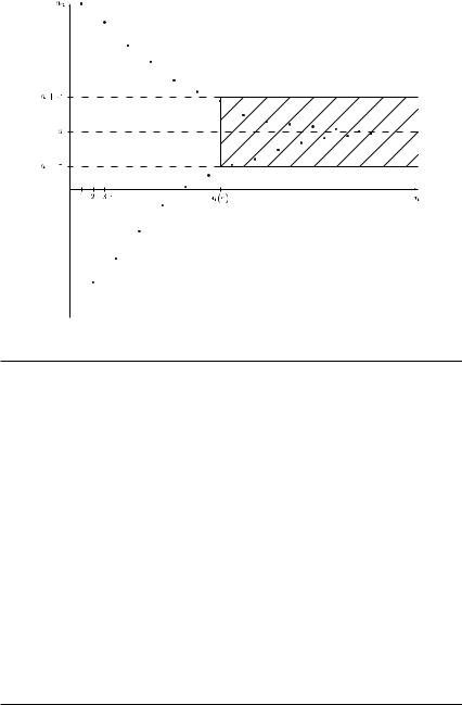
Definition 2.6 A finite number a is called the limit of a sequence {an} if, for any given ε > 0, there exists an index n(ε) such that

|an − a| < ε for all n ≥ n(ε).

To indicate that number a is the limit of sequence {an}, we write

lim an = a.

n→∞

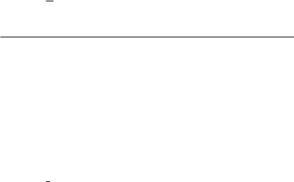
The notion of the limit a is illustrated in Figure 2.1. Sequence {an} has the limit a, if there exists some index n(ε) (depending on ε) such that the absolute value of the difference between the term an and the limit a becomes smaller than the given value ε for all terms an with n ≥ n(ε), i.e. from some n on, the terms of the sequence {an} are very close to the limit a. If ε becomes smaller, the corresponding value n(ε) becomes larger. To illustrate the latter definition, we consider the following example.

66 Sequences; series; finance

Figure 2.1

The limit a of a sequence {an}.

Example 2.7 Let sequence {an} be given with

an = 1 +

i.e. we get

a1 = 2, a2 =

a3 =

a4 =

, . . . .

The terms of sequence {an} tend to number one. For example, if ε = 1/100, we get

|an − 1| = 1 + n2

− 1

= n2

< 100 ,

which is satisfied

for n

≥

n(ε)

≥

11 have an absolute difference

11, i.e. all terms an with n

from the limit a = 1 smaller than ε = 1/100.

If we choose a smaller value of ε, say ε = 1/10, 000, we obtain for n ≥ n(ε) = 101 only that

1		1
\|an − 1\| =		<		,
	n2		10, 000

i.e. all terms an with n ≥ n(ε) = 101 have an absolute difference smaller than ε = 1/10, 000 from the limit a = 1 of the sequence. Note, however, that independently of the choice of ε, there are infinitely many terms of the sequence in the interval (a − ε, a + ε).

Sequences; series; finance 67

The definition of a limit is not appropriate for determining its value. It can be used to confirm that some (guessed) value a is in fact the limit of a certain sequence.

Example 2.8 Consider the sequence {an} with

n − 2

We get

1 − 2

= −

, a

2 − 2

0, a

3 − 2

, . . . .

3 = 2

For larger values of n, we obtain e.g.

a50 =		48		≈ 0.466,	a100 =		98	≈ 0.483,	a1,000 =	998		≈ 0.498,
	103					203				2, 003

and we guess that a = 1/2 is the limit of sequence {an}. To prove it, we apply Definition 2.6 and obtain

| n − | =

− 2

(2n

a a

−

< ε.

= 4n

By taking the reciprocal

values of the latter inequality, we get

4n + 6

7ε

which can be rewritten as

7 − 6ε

n >		,

	4ε

i.e. in dependence on ε we get a number n = n(ε) such that all terms an with n ≥ n(ε) deviate from a by no more than ε. For ε = 10−2 = 0.01, we get

n > 7 − 6 · 0.01 = 173.5, 4 · 0.01

i.e. we have n(ε) = 174 and from the 174th term on, all terms of the sequence deviate by less than ε = 0.01 from the limit a = 1/2. If ε becomes smaller, the number n(ε) increases, e.g. for ε = 10−4 = 0.0001, we get

n > 7 − 6 · 0.0001 ≈ 17, 498.5, 4 · 0.0001

i.e. n(ε) = 17, 499.

68 Sequences; series; finance

If a sequence has a limit, then it is said to converge. Now we are able to give a first convergence criterion for an arbitrary sequence.

THEOREM 2.1 A bounded and monotone (i.e. increasing or decreasing) sequence {an} converges.

We illustrate the use of Theorem 2.1 by the following example.

Example 2.9 Consider the recursively defined sequence {an} with

a1 = 1 and an+1 = 3 · an, n N.

First, we prove that this sequence is bounded. All terms are certainly positive, and it is sufficient to prove by induction that an < 3 for all n N. In the initial step, we find that a1 = 1 < 3. Assuming an < 3 in the inductive step, we obtain

an+1 = 3 · an < √3 · 3 = 3

for all n N. Therefore, implication

an < 3 = an+1 < 3

is true. Hence, sequence {an} is bounded by three.

To show that sequence {an} is increasing, we may investigate the quotient of two successive terms (notice that an > 0 for n N) and find

	=			=
an					an
			an
an+1		√3 · an				3	> 1.

The latter inequality is obtained due to an < 3. Therefore, an+1/an > 1 and thus an+1 > an, i.e. sequence {an} is strictly increasing. Since sequence {an} is bounded by three, we have found by Theorem 2.1 that sequence {an} converges.

Now, we give a few rules for working with limits of sequences.

THEOREM 2.2 Assume that the limits

nlim	an = a and	nlim bn = b
→∞		→∞

exist. Then the following limits exist, and we obtain:

(1)	nlim	(an ± c) = nlim (an) ± c = a ± c for constant c R;
	→∞	→∞
(2)	nlim	(c · an) = c · a for constant c R;
	→∞	(an ± bn) = a ± b;
(3)	nlim	(an ± bn) = a ± b;
	→∞

Sequences; series; finance 69

(4) lim (an · bn) = a · b;

n→∞

(5) nlim	an		=	a	(b = 0).
	b	n		b
→∞

We illustrate the use of the above rules by the following example.

Example 2.10 Let the sequences {an} and {bn} with

n =

2n2 + 4n − 1

3n2 − 1

5n2 + 10

= n3 + 2n

be given. Then

2n2 + 4n − 1

2 + n4

−

lim a

lim

→∞

+ 10

→∞

n2 5 + n2

2 + nlim

nlim

− nlim

−

→∞

lim

n→∞

+ n→∞ n2

Similarly, we get

3n2 − 1

n2 3 −

lim bn

lim

n→∞

= n→∞ n3 + 2n = n→∞ n2 n + n2

nlim

3 − nlim

−

→∞

lim

2 =

lim n

0 =

→∞

n→∞

+ n→∞ n

Consider now sequence {cn} with

cn = an + bn,

n N.

Applying the given rules for limits, we get

nlim cn

= nlim

+ nlim

bn =

+ 0 =

→∞

As an alternative to the above calculation, we can also first determine the nth term of sequence {cn}:

n =

n +

2n2 + 4n − 1

3n2 − 1

5(n2 + 2)

+ n(n2 + 2)

+ 195 n2 − 51 n − 1

51 · (2n3

+ 4n2 − n) + 3n2 − 1

52 n3

n3 + 2n

70 Sequences; series; finance

Determining now

lim cn

n→∞

we can get the same result as before.

In generalization of the above example, we can get the following result for p, q N:

+ −

+ +

for p < q

lim

apn

+ ap−1n −

+ . . . + a1n + a0

for p

q 1

n→∞ bqn

bq 1n

−

. . .

b1n b0

for p > q.

∞

This means that, in order to find the above limit, we have to check only the terms with the largest exponent in the numerator and in the denominator.

Example 2.11 We consider sequence {an} with

an =

+ 2,

n N.

7n 3

−

Then

−

→∞

−

→∞

nlim

+ 2& =

nlim

+ nlim 2

+ 2 =

+ 2 = 49 .

107

We finish this section with some frequently used limits.

Some limits
(1)	nlim	1			= 0;

			n
	→∞	an = 0 for \|a\| < 1;
(2)	nlim	an = 0 for \|a\| < 1;
	→∞
(3)	nlim		n
			n
		√c = 1 for constant c R, c > 0;
	→∞
(4)	nlim		n
			n
		√n = 1;
	→∞		an
(5)	nlim		an		= 0;
(5)	nlim		n	!	= 0;
	→∞			!
(6)	nlim		nk			= 0;
(6)	nlim		n	!		= 0;
	→∞			!

Sequences; series; finance 71

(7) lim n! = 0;

n→∞ nn

(8) lim 1 + 1 n = e.

n→∞ n

From limits (5) up to (7), one can conclude that the corresponding term in the denominator grows faster than the term in the numerator as n tends to infinity.

2.2 SERIES

2.2.1 Partial sums

We start this section with the introduction of the partial sum of some terms of a sequence.

Definition 2.7 Let {an} be a sequence. Then the sum of the first n terms

sn = a1 + a2 + . . . + an = ak

k=1

is called the nth partial sum sn.

Example 2.12 Consider the sequence {an} with
2
an = 3 + (−1)n ·		, n N,
an = 3 + (−1)n ·	n	, n N,
i.e.
							2			=	7				1	=	7
a1 = 3 − 1 · 2 = 1, a2 = 3 + 1 = 4, a3 = 3 −													, a4	= 3 +					, . . . .
a1 = 3 − 1 · 2 = 1, a2 = 3 + 1 = 4, a3 = 3 −									3			3	, a4	= 3 +	2		2		, . . . .
Then we get the following partial sums:
s1 = a1 = 1, s2 = a1 + a2 = 1 + 4 = 5, s3 = a1 + a2 + a3 = 1 + 4 +															7	=	22
																				,
															3			3		,
s4 = a1 + a2 + a3 + a4 = 1 + 4 +			7	7			65
				+		=		, . . . .
			3	+	2	=	6	, . . . .

For special types of sequences (namely, arithmetic and geometric sequences), we can easily give the corresponding partial sums as follows.

72 Sequences; series; finance

THEOREM 2.3 The nth partial sum of an arithmetic sequence {an} with an = a1 + (n − 1) · d is given by

sn =	n	· (a1 + an) =	n	· [2a1 + (n − 1)d] .

	2		2

The nth partial sum of a geometric sequence {an} with an = a1 · qn−1 and q = 1 is given by

1 − qn sn = a1 · 1 − q .

Example 2.2 (continued) We determine the total car production within the first twelve months of production. To this end, we have to determine the twelfth partial sum s12 of an arithmetic sequence with a1 = 750 and d = 20. We obtain

s12 = n · (2a1 + 11 · d) = 6 · (1, 500 + 11 · 20) = 10, 320, 2

i.e. the total car production within the first year is equal to 10,320.

Example 2.13 Consider a geometric sequence with a1										= 2 and q = −4/3, i.e. the next
four terms of the sequence are
8			32				128			512
a2 = −		,	a3 =		,	a4 = −		,	a5 =			.
	3			9			27				81

According to Theorem 2.3, we obtain the fifth partial sum as follows:

s5	= a1	· 1− q		= 2 ·		−		−	4	= 2 ·	−	7	= 2 · 243	· 7	=	81 .
			1 q5		1		(		34 )5	1		− 1024243	1267	3		362
			−		1 − (− 3 )							3

Example 2.4 (continued) We wish to know what will be the total production of DVD players from the beginning of 2001 until the end of 2012. We apply the formula for the partial sum of a geometric sequence given in Theorem 2.3 and obtain

12 =

1 ·

1 − q =

1 − 1.1 =

−0.1

−

≈

1 − qn

20, 000

1 − 1.112

20, 000

1.112

427, 686.

The firm will produce about 427,686 DVD players in the years from 2001 until 2012.

Example 2.14 Two computer experts, Mr Bit and Mrs Byte, started their jobs on 1 January 2002. During the first year, Mr Bit got a fixed salary of 2,500 EUR every month and his

Sequences; series; finance 73

salary rises by 4 per cent every year. Mrs Byte started with an annual salary of 33,000 EUR, and her salary rises by 2.5 per cent every year.

First, we determine the annual salary of Mr Bit and Mrs Byte in 2010. Mr Bit got 30,000 EUR in 2002, and in order to determine his salary in 2010, we have to find the term a9 of a geometric sequence with a1 = 30, 000 and q = 1.04:

a9 = 30, 000 · 1.048 = 41, 057.07.

To find the salary of Mrs Byte, we have to find the term b9 of a sequence with b1 = 33, 000 and q = 1.025:

b9 = 33, 000 · 1.0258 = 40, 207.30.

In 2010, the annual salary of Mr Bit will be 41,057.07 EUR and the annual salary of Mrs Byte will be 40,207.30 EUR. Next, we wish to know which of them will earn more money over the years from 2002 until the end of 2010. To this end, we have to determine the partial sums of the first nine terms of both sequences. For sequence {an}, we obtain

1 − q9

30, 000

1 − 1.049

≈

317, 483.86.

−

q =

−

1.04

For sequence {bn}, we obtain

1 − q9

33, 000

1 − 1.0259

≈

328, 499.12.

−

q =

−

1.025

Hence, Mrs Byte will earn about 11,000 EUR more than Mr Bit over the nine years.

2.2.2 Series and convergence of series

Definition 2.8 The sequence {sn} of partial sums of a sequence {an} is called an

(infinite) series.

A series {sn} is said to converge if the sequence {sn} has a limit s. This value

	n	∞
s = nlim
s = nlim	sn = nlim	ak = ak
→∞	→∞ k=1	k=1

is called the sum of the (infinite) series {sn}.

If {sn} does not have a limit, the series is said to diverge.

Example 2.15 We investigate whether the series {sn} with

n

	2
sn = k=1 k2 , n N,

74 Sequences; series; finance

converges. To this end, we apply Theorem 2.1 to the sequence of partial sums {sn}. First, we note that this sequence {sn} is strictly increasing, since every term ak = 2/k2 is positive for all k N and therefore, sn+1 = sn + an > sn. It remains to prove that sequence {sn} of the partial sums is also bounded. For k ≥ 2, we obtain the following estimate of term ak :

ak =

≤

k2 − k

k(k − 1)

= 2

k − 1

−

Then we obtain the following estimate for the nth partial sum sn:

sn = k

= 2 + k

≤

2 + 2 k

−

k − 1

= 2 + 2

'2 1

− 2

1 1

− 3

4 1 1

− 4

+ . . . + n

1 1

− n (

−

	1
= 2 + 2 ·	1 −		≤ 4.
		n

The last equality holds since all terms within the brackets are mutually cancelled except the first and last terms. Thus, the strictly increasing sequence {sn} of partial sums is also bounded. From Theorem 2.1, series {sn} with

n 2 sn = k=1 k2

converges.

THEOREM 2.4 (Necessary convergence criterion) Let the series {sn} with

sn = ak , n N,

k=1

be convergent. Then

lim an = 0.

n→∞

The condition of Theorem 2.4 is not sufficient. For instance, let us consider the so-called harmonic series {sn} with

n 1

sn = , n N.

k=1 k

Next, we show that this series does not converge although

nlim	an = nlim	1	= 0.
		n
→∞	→∞

Sequences; series; finance 75 Using the fact that for n ≥ 4, n N, there exists a number k N such that 2k+1 ≤ n < 2k+2,

we obtain the following estimate for the nth partial sum sn:
				1		1									1	1
sn = 1 +						+		+ · · · +								+ · · · +
sn = 1 +				2		+	3	+ · · · +						2k+1		+ · · · +	n			+	2k + 1		+ · · · + 2k+1 + · · · + n
		= 1 + 2 +						3 + 4				+			5	+ · · · + 8				+	2k + 1		+ · · · + 2k+1 + · · · + n
				1				1		1					1	1					1				1	1
		> 1 +		1				1				1			+ · · · + 2k ·				1		= 1 +	1		1		1
						+ 2		·		+ 4 ·													+		+ · · · +
				2		+ 2		·	4	+ 4 ·		8						2k+1				2	+	2	+ · · · +	2

																							+
																						k		1 summands
Consequently, we get
s		>	2		k + 1			=			k + 3		.
s		>											.
	n	2 +				2				2

Since for any (arbitrarily large) k N, there exists a number n N such that sn can become arbitrarily large, the partial sum sn is not bounded. Thus, the sequence of the partial sums {sn} does not converge.

Definition 2.9 Let {an} be a geometric sequence. The series {sn} with

n	n

sn = ak =	a1 · qk−1
k=1	k=1

is called a geometric series.

For a geometric series, we can easily decide whether it converges or not by means of the following theorem.

THEOREM 2.5 A geometric series {sn} with a1 = 0 converges for |q| < 1, and we obtain

1 − qn

qk−1

1 ·

lim s

lim

lim a

n→∞

n = n→∞ k

= n→∞

1 − q

For |q| ≥ 1, series {sn} diverges.

Example 2.16 Consider the series {sn} with

sn = k 1 2 ·	− 2		−	, n N.
n	1	k		1

=

76 Sequences; series; finance

This is a geometric series with a1 = 2 and q = −1/2. Applying Theorem 2.5 we find that this series converges, since |q| = 1/2 < 1, and we obtain

		sn	=	a1	=	2	=	2	=	4
	→∞		=	1 − q	=	1 − − 2	=	2	=	3
lim						1		3		.
n						1		3

A first general criterion for checking convergence of a series has already been discussed in connection with sequences (see Theorem 2.1). If the sequence of the partial sums is bounded and monotone, the series {sn} certainly converges. We consider a similar example to Example 2.15, which however uses Theorem 2.5 for estimating the terms sn.

Example 2.17 We consider the series {sn} with

n N.

sn = k

(k − 1)!

Determining the first partial sums, we obtain

s1 =

= 2, s2 = s1 +

= 2 + 2

= 4, s3

= s2 +

= 4 + 1 = 5,

s4 = s3 +

= 5 +

, . . . .

Since

ak =

> 0

for all k N,

(k − 1)!

sequence {sn} of the partial sums is strictly increasing. To check whether sequence {sn} is bounded, we first obtain for k ≥ 3:

ak =

≤

(k − 1)!

1 · 2 · 3 · . . . · (k − 1)

1 · 2 · 2 · . . . · 2

2k−3

−

2 factors

Denoting ak = 1/2k−3, k ≥ 3, the following estimate holds for n ≥ 3:

sn ≤ a1 + a2 + a3 + . . . + an

n−2

= 2 +

+ k

2k−3

= 4 + k

2k−1

= + k 1 2

k−1

≤ + k 1

= +

1 −

21 =

n−2

∞

k−1

Sequences; series; finance 77

i.e. each partial sum sn with n ≥ 3 is no greater than six (notice that s1 = 2 and s2 = 4). In the above estimate of sn, we have used the sum of a geometric series given in Theorem 2.5. Thus, sequence {sn} is strictly increasing and bounded. From Theorem 2.1, the series {sn} with

	n
				2
sn =	=	1	(k	−	1)	!
k		1		−		!

converges.

Definition 2.10 A series {sn} with

sn = ak

k=1

is called alternating if the signs of the terms ak alternate.

We can give the following convergence criterion for an alternating series.

THEOREM 2.6 (Leibniz’s criterion) Let {sn} with

sn = ak

k=1

be an alternating series. If the sequence {|ak |} of the absolute values is decreasing and

lim ak = 0,

k→∞

series {sn} converges.

Example 2.18 We consider the series {sn} with

		n		n	(−1)k+1
s	n =		k =		(−1)k+1	· 3
s		a					,	n	N.
		k=1		k=1	k
		k=1		k=1

This is an alternating series with

s1 = a1 = 3, s2 = s1 + a2 = 3 −											3			3			= s2 + a3 =			3		5
													=			, s3					+ 1 =			,
												2	=		2	, s3				2	+ 1 =		2	,
s4 = s3 + a4 =			5		3	7
				−		=			, . . .
			2	−	4	=		4	, . . .
First, due to
a	a			3			3			3k − 3(k + 1)								3			< 0,
a	a	k \| = k			1	− k			=								= − k(k		1)		< 0,
\|	k+1\| − \|	k \| = k		+	1	− k			=		k(k			+	1)		= − k(k	+	1)
				+										+				+

78 Sequences; series; finance

sequence {|ak |} is strictly decreasing. Furthermore,

lim (−1)k+1 · 3 = 0,

k→∞ k

and thus by Theorem 2.6, series {sn} converges.

We now present two convergence criteria which can be applied to arbitrary series.

THEOREM 2.7 (quotient criterion) Let {sn} be a series with

sn =	ak .
k=1
Then:
(1) If
Q	lim	ak+1
Q	lim	ak+1
	= k→∞	ak	< 1,

series {sn} converges.

(2)If Q > 1, series {sn} diverges.

(3)For Q = 1, a decision is not possible by means of the quotient criterion.

Example 2.19 We investigate whether the series {sn} with

n

	k
sn = k=1 4k , n N,

converges. Applying the quotient criterion, we get with ak = k/4k

ak+1

· 4k

k + 1 .

4k+1 k

Therefore,

lim

ak+1

lim

k + 1

1 < 1.

= k→∞

Thus, the given series converges.

Example 2.20 Consider the series {sn} with

n	3k3

sn =	2k	, n N.
k=1

Sequences; series; finance 79

Using the quotient criterion, we get

2k+1

3k3

2 ·

ak+1

· 2k

3k2 + 3k + 1

and

ak+1

1 .

lim

= k→∞

Thus, the series considered

converges.

THEOREM 2.8 (root criterion)

Let {sn} be a series with

sn =

ak .

k=1

Then:

(1) If

R = k→∞

k |

< 1,

lim

series {sn} converges.

(2)If R > 1, series {sn} diverges.

(3)For R = 1, a decision is not possible by means of the root criterion.

Example 2.21 Let the series {sn} with


	n	k
	sn = k=1	k
	sn = k=1	2k , n N,

be given. In order to investigate it for convergence or divergence, we apply the root criterion and obtain

k k

|ak | = √ak

√k.

Further,

lim

k a

lim

√k

lim

√k

= 2

= 2 ·

R = k→∞

k | = k→∞

· k→∞

The latter result is obtained using the given limit (see limit (4) at the end of Chapter 2.1.2)

	√
klim	k	k = 1.
klim		k = 1.
→∞

Hence, the series considered converges due to R < 1.

80 Sequences; series; finance

Example 2.22 Consider the series {sn} with

n = k 1	k	·		−
n		k2
	k + 1				k ,
s			2		k ,	n N.

To check {sn} for convergence, we apply the root criterion and obtain

= k→∞ | k | = k→∞

· −

k + 1

R lim

lim

2 k

→∞

= klim

1 +

· klim

1 +

· e > 1.

The latter equality holds due to limit (8) given at the end of Chapter 2.1.2. Hence, since R > 1, series {sn} diverges.

2.3 FINANCE

In this section, we discuss some problems arising in finance which are an application of sequences and series in economics. Mainly we use geometric and arithmetic sequences and partial sums of such sequences. In the first two subsections, we investigate how one payment develops over time and then how several periodic payments develop over time. Then we consider some applications of these considerations such as loan repayments, evaluation of investment projects and depreciation of machinery.

2.3.1 Simple interest and compound interest

We start with some notions. Let P denote the principal, i.e. it is the total amount of money borrowed (e.g. by an individual from a bank in the form of a loan) or invested (e.g. by an individual at a bank in the form of a savings account). Interest can be interpreted as money paid for the use of money. The rate of interest is the amount charged for the use of the principal for a given length of time, usually on a yearly (or per annum, abbreviated p.a.) basis, given either as a percentage ( p per cent) or as a decimal i, i.e.

i = p =) p % 100

If we use the notation i for the rate of interest, then we always consider a decimal value in the rest of this chapter, and we assume that i > 0.

In the following, we consider two variants of interest payments. Simple interest is interest computed on the principal for the entire period it is borrowed (or invested). In the case of simple interest, it is assumed that this interest is not reinvested together with the original capital. If a principal P is invested at a simple interest rate of i per annum (where i is a decimal) for a period of n years, the interest charge In is given by

In = P · i · n.

Sequences; series; finance 81

The amount A owed at the end of n years is the sum of the principal borrowed and the interest charge:

A = P + In = P + P · i · n = P · (1 + i · n).

Simple interest is usually applied when interest is paid over a period of less than one year.

If a lender deducts the interest from the amount of the loan at the time the loan is made, the loan is said to be discounted. In this case, the borrower receives the amount P (also denoted as proceeds) given by

P = A − A · i · n = A · (1 − i · n),

where A · i · n is the discount and A is the amount to be repaid at the end of the period of time (also known as the maturity value). We emphasize that in the case of a discounted loan, interest has to be paid on the total amount A (not on the proceeds P) at the beginning of the period.

Next, we assume that at the end of each year, the interest which is due at this time is added to the principal so that the interest computed for the next year is based on this new amount (of old principal plus interest). This is known as compound interest. Let Ak be the amount accrued on the principal at the end of year k. Then we obtain the following:

A1 = P + P · i = P · (1 + i),

A2 = A1 + A1 · i = A1 · (1 + i) = P · (1 + i)2,

A3 = A2 + A2 · i = A2 · (1 + i) = P · (1 + i)3,

and so on. The amount An accrued on a principal P after n years at a rate of interest i per annum is given by

An = P · (1 + i)n = P · qn.

(2.1)

The term q = 1 + i is also called the accumulation factor. Note that the amounts Ak , k = 1, 2, . . ., are the terms of a geometric sequence with the common ratio q = 1 + i. It is worth noting that in the case of setting A0 = P, it is a geometric sequence starting with k = 0 in contrast to our considerations in Chapter 2.1, where sequences began always with the first term a1. (However, when beginning with A0, one has to take into account that An is already the (n + 1)th term of the sequence.) The above formula (2.1) can be used to solve the following four basic types of problems:

(1)Given the values P, i and n, we can immediately determine the final amount An after n years using formula (2.1).

(2)Given the final amount An, the interest rate i and the number of years n, we determine the principal P required now such that it turns after n years into the amount An when the rate of interest is i. From formula (2.1) we obtain

P =		An		.
P =	(1	+	i)n	.
		+

82 Sequences; series; finance

(3)Given the values n, P and An, we determine the accumulation factor q and the rate of interest i, respectively, which turns principal P after n years into the final amount An. From formula (2.1) we obtain

An	= (1 + i)n.	(2.2)
P

Solving for i, we get

nAn = 1 + i P

i = n An − 1. P

(4)Given the values An, P and i, we determine the time n necessary to turn principal P at a given rate of interest i into a final amount An. Solving formula (2.2) for n, we obtain


An		= n · ln(1 + i)
ln
	P
	n	=	ln An − ln P			.

			ln(1	+	i)

We give a few examples to illustrate the above basic problems.

Example 2.23 What principal is required now so that after 6 years at a rate of interest of 5 per cent p.a. the final amount is 20,000 EUR?

This is a problem of type (2) with n = 6, i = 0.05 and A6 = 20, 000. We obtain:

P =		A6		=		20, 000		= 14, 924.31 EUR
P =	(1	+	i)6	=	(1	+	0.05)6	= 14, 924.31 EUR
		+				+

i.e. the principal required now is equal to 14,924.31 EUR.

Example 2.24 How long will it take to double a principal of 20,000 EUR when the interest rate is 6 per cent p.a.?

This is a problem of type (4). Using P = 20, 000, An = 40, 000 and i = 0.06, we obtain

n = ln 40, 000 − ln 20, 000 ≈ 11.9 ln 1.06

i.e. it takes about 11.9 years to double the principal.

Often, we do not have an annual period for interest payments, i.e. compounding takes place several times per year, e.g.

(1)semi-annually – there are 2 interest payments per year, namely after every six months;

(2)quarterly – there are 4 payments per year, namely one after every three months;

(3)monthly – there are 12 payments, namely one per month;

Sequences; series; finance 83

(4)daily – compounding takes place 360 times per year (in this section, we always count 12 months with 30 days each).

Note that in all cases, it is assumed that interest payment is made after equal length periods. In the case of m interest payments per year, the rate of interest per payment period is equal to i/m, where i is as before the per annum rate of interest as a decimal, and the number of interest payments within a period of n years is equal to n · m. Denoting by An,m the amount at the end of n years with m interest payments per year, formula (2.1) changes into

i	n m
i	· .
An,m = P · 1 + m	· .	(2.3)

Example 2.25 Mrs Rich wishes to invest 15,000 EUR. The bank offers a rate of interest of 6 per cent p.a.

We compute the resulting amount of money at the end of four years when compounding takes place annually, quarterly and monthly. We use formulas (2.1) and (2.3) with P = 15, 000 EUR and i = 0.06.

In the case of annual compounding, we get

A4 = P · (1 + i)4 = 15, 000 · (1 + 0.06)4 = 18, 937.15 EUR.

Hereafter, we use the equality sign although all amounts are rounded to two decimal places. When compounding takes place four times per year, we compute A4,4 and obtain


	i		4 4
A4,4 = P · 1 +			·			= 15, 000 · 1.01516 = 19, 034.78 EUR.

	4
Finally, when compounding takes place monthly, we compute A4,12 and obtain
A4,12 = P · 1 +			i		4 12

				·			= 15, 000 · 1.00548 = 19, 057.34 EUR.
		12

If the compounding takes place several times per year or if the interest rate is not constant over time, one is often looking for the effective rate of interest ieff . This is the rate of interest necessary to turn the principal into the final amount when compounding takes place annually. In the case of m interest payments per year at a per annum rate i of interest, there is an interest payment of i/m per interest payment period, and we obtain from formula (2.3)

(1 + ieff ) = 1			i	m
	+

			m
ieff = 1			i	m
	+			− 1.

		m

84 Sequences; series; finance

Similarly, if there are different per annum rates of interest i1, i2, . . . , in with an annual compounding, we obtain from formula (2.1)

(1 + ieff )n = (1 + i1) · (1 + i2) · . . . · (1 + in)

ieff = n (1 + i1) · (1 + i2) · . . . · (1 + in) − 1.

Example 2.26 A bank offers a rate of interest of 6 per cent p.a. compounded quarterly. What is the corresponding effective rate of interest ieff ?

Since m = 4, the rate of interest per period is

i = 0.015, 4

and we obtain

ieff = (1.015)4 − 1 = 0.06136355

i.e. the offer from the bank corresponds to an effective rate of interest of 6.14 per cent p.a.

Finally we briefly discuss a mixture of simple and compound interest. This is used when interest is paid not only for complete interest periods. We illustrate this by the following example.

Example 2.27 Assume that Mr Happy gives 10,000 EUR to a bank on 15 November 2001 and that he would like to have money back on 20 February 2005. The bank offers a constant rate of interest of 4 per cent p.a. compounded annually.

We can apply the formula for compound interest for the years 2002, 2003 and 2004, but for the parts of 2001 and 2005, we apply the formula for simple interest. Remembering our assumption that every month consists of 30 days, the bank pays interest for 45 days in 2001 and for 50 days in 2005.

Therefore, the amount at the end is given by

A = 10, 000 · 1 + 0.04 ·	45	· (1	+ 0.04)3 · 1 + 0.04 ·	50
	360			360

= 11, 367.69 EUR .

In the above calculations, simple interest is computed for the 45 days from 16 November to 31 December 2001 (i.e. the principal is multiplied by 1 + 0.04 · 45/360) and for the 50 days from 1 January to 20 February 2005 (i.e. the amount at the end of 2004 is multiplied by 1 + 0.04 · 50/360). For the three intermediate years from 2002 to 2004, we apply the compound interest formula, which leads to the factor (1 + 0.04)3.

Sequences; series; finance 85

2.3.2 Periodic payments

In the previous subsection, we considered the computation of the future value of one investment when a fixed amount of money is deposited in an account that pays interest compounded periodically. In many situations, there are periodic payments (i.e. deposits or withdrawals) and the question is which amount is accrued (or left over) after a number of payment periods. Such situations occur, for example, in connection with annual life insurance premiums, monthly deposits at a bank, loan repayments, sinking funds and so on.

The notion annuity is used in the following for a sequence of (usually equal) periodic payments. Here we consider only the case when payment periods and the periods for interest payments coincide. Moreover, the interest is always credited at the end of a payment period.

First, we consider a so-called ordinary annuity, where the payments (deposits) are made at the same time the interest is credited, namely at the end of the period. We mark all values by the superscript ‘E’ which stands for ‘end of the period’.

Annual payments

Again, we first consider the case of annual payments r. The amount of an annuity is the sum of all payments (deposits) made plus all interest accumulated. Next, we compute the amount of an annuity AEn , i.e. the total amount after n annual payment periods. Denoting by Dk the amount resulting from the kth deposit at the end of n years, we get

AEn = D1 + D2 + . . . + Dn = r · (1 + i)n−1 + r · (1 + i)n−2 + . . . + r · (1 + i) + r

= r · 1 + (1 + i) + . . . + (1 + i)n−1 .

The term in brackets on the right-hand side represents the partial sum sn of a geometric sequence with a1 = 1 and q = 1 + i. Note that the kth deposit accumulates the value Dk , where the payments are compounded over n − k years. We use the formula for the partial sum of the first n terms of a geometric sequence and obtain

+ · · · +

i)n−1

1 − (1 + i)n

(1 + i)n − 1

−

i) =

−

Thus, we have shown the correctness of the following theorem.

THEOREM 2.9 (amount of an annuity) If an amount r is deposited at the end of each year at a per annum rate of interest i, the amount AEn of the annuity after n annual payments is

AE	=	r	·	(1 + i)n − 1	.	(2.4)

n				i

The present value of an annuity is the amount of an annuity discounted over the whole time period, i.e. it is the amount of money needed now so that after depositing this amount for a period of n years at a per annum rate of interest of i, the amount of an annuity AEn results. We

86 Sequences; series; finance

get

(1 + i)n − 1

= (1

i)n

= (1

i)n

= r · (1 + i)−n · [(1 + i)n − 1] = r · 1 − (1 + i)−n .

In connection with periodic withdrawals the present value PnE has an important meaning. It is the amount of money needed now so that, if it is invested at a per annum rate of interest i, n equal money amounts r can be withdrawn at the end of each year without any money left over at the end.

To illustrate this, let us argue that the sum of the present values of the individual withdrawals is indeed equal to PnE. Assume that the withdrawals are made at the end of each year and let PVk be the present value of the kth withdrawal. Then

PVk = r · (1 + i)k .

Summing up, we get

PV = PV1 + PV2 + · · · + PVn

= r ·

+ r

+ · · · + r ·

i)2

i)n

= r · (1 + i)n · 1 + (1 + i) + · · · + (1 + i)n−1

i)−n

1 − (1 + i)n

(1 + i)−n − 1

−

=r · 1 − (1 + i)−n = PE, i n

i.e. the sum of the present values of all the n withdrawals corresponds to PnE. Therefore, we have proved the following theorem.

THEOREM 2.10 (present value of an annuity)					If r represents the withdrawal at the end of
each of n years, the present value PE of an annuity at a per annum rate of interest i is
				n
PE	r	·	1 − (1 + i)−n	.	(2.5)

n =			i

As a consequence, we do not need to distinguish between periodic deposits and withdrawals in the sense that formulas follow the same pattern. When considering periodic deposits, we are usually interested in the amount of an annuity AEn , and when considering periodic withdrawals we are interested in the present value of an annuity PnE.

Next, we discuss the case when the payments are made at the beginning of the period while interest is still credited at the end. We mark the corresponding values by the superscript ‘B’ which stands for ‘beginning of the period’. Notice that this is not an ordinary annuity.

Sequences; series; finance 87

First, we discuss the modification of the formula for the amount of the annuity ABn . The difference from the previous case is that for each deposit, interest is credited for one more period, i.e. the kth deposit accumulates interest over n − k + 1 years. Let Dk be the amount at the end of n years which results from the kth deposit. Then Dk = r · (1 + i)n−k+1. Therefore, we get

AnB = Dn−1 + Dn−2 + . . . + D1 = r · (1 + i) + r · (1 + i)2 + . . . + r · (1 + i)n

=r · (1 + i) · 1 + (1 + i) + (1 + i)2 + . . . + (1 + i)n−2 + (1 + i)n−1

=r · (1 + i) · (1 + i)n − 1 .

By the above computations we have found that ABn = (1 + i) · AEn which reflects the fact that for each deposit, interest is credited for one more year in comparison with deposits at the end of each year.

Correspondingly, the present value PnB for a period of n years, i.e.

PnB =		1		· AnB = r · (1 + i) ·
PnB =	(1	+	i)n	· AnB = r · (1 + i) ·
		+

is obtained by discounting the amount of an annuity

1 − (1 + i)−n

We now discuss some basic types of problems connected with periodic payments (deposits or withdrawals). Here we consider only the case when payments are made at the end of each year and interest is credited at the same time. In the above formulas we have used the values PnE, AEn , r, i and n. Among these values, at least two (or even three) must be given for each problem type, and we are looking for one of the remaining values.

(1)Given the per annum rate of interest i and the number of years n, we are looking for the amount of the annuity AEn . This problem arises when annual deposits are made in an account, rate of interest as well as the time period are known in advance, and we

wish to determine the amount in the account at the end of n years. In this case, we can immediately apply formula (2.4).

(2)Given the values r, i and n, we are looking for the present value of the annuity PnE. This type of problem arises when periodic withdrawals are made, and we wish to know the

current amount required to guarantee the n withdrawals such that no money is left over at the end when the time period and rate of interest are known. In this case, we can immediately apply formula (2.5).

(3)Given the values AEn , i and n, we are looking for the annual payment r to get the final amount AEn provided that the time period of the periodic payments and the rate of interest are known. From formula (2.4), we obtain

r = AnE ·	i
		.
	(1 + i)n − 1

(4) Given the values AEn , r and i, we are looking for the time period n which is required to accumulate the final amount AEn by periodic payments of an amount r at a given constant rate of interest i. In this case, we obtain

AE · i = (1 + i)n − 1

n r

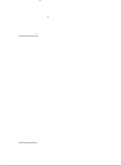
88Sequences; series; finance which can also be written as

(1 + i)n = 1 + AE · i .

n r

Taking the natural logarithm on both sides, we obtain

ln(1 + i)n = ln 1 + AE · i .

n r

Solving the latter equation for n and using the equality ln(1 + i)n = n · ln(1 + i), we get

	ln	1 + AnE · ri
n =		ln(1 + i)		.	(2.6)

(5)Given the values AEn , n and r, we wish to determine the accumulation factor q resp. the per annum rate of interest i = q − 1. This is, from a mathematical point of view, a more

complicated problem. First, from formula (2.4), we obtain

AE · i = r · (1 + i)n − 1 .

This yields

		AnE · (1 + i) − AnE = r · (1 + i)n − r
r · (1 + i)n − AnE · (1 + i) + (AnE − r) = 0
	AE		AE
(1 + i)n −	n	· (1 + i) +	n	− 1 = 0.
	r		r

Now, the problem corresponds to finding the zeroes of a polynomial of degree n in the variable q = 1 + i and in general, we cannot solve this equation for q. Therefore, we have to apply approximation methods for finding a root of this equation greater than one (remember that only values q = 1 + i > 1 are of interest). In Chapter 4, we discuss some procedures for finding a zero of a function numerically. However, there is another difficulty for big values of n: possibly there is no uniquely determined solution q > 1.

Similarly to problems of type (3), (4) and (5), we can formulate the corresponding problems, where the amount of an annuity AEn has been replaced by the present value of an annuity PnE. As an example, for the problem of type (3), this gives the equality

r = PnE ·	i
r = PnE ·	1 − (1 + i)−n .	(2.7)

Analogously, one can formulate the corresponding problems for the case when the payments are made at the beginning of the years. This is left as an exercise for the reader. We illustrate the solution of the basic problems mentioned above by some examples.

Example 2.28 What is the principal required now in order to be able to withdraw 3,000 EUR at the end of each of ten years (beginning at the end of the first year) so that no money is left over after these ten years provided that a rate of interest of 5 per cent p.a. is offered?

Sequences; series; finance 89

This question is the same as asking for the present value of an annuity P10E with r = 3, 000 and i = 0.05. We obtain

1 − (1 + i)−10

3, 000

1 − (1 + 0.05)−10

23, 165.20 EUR,

0.05

i.e. the principal required now to ensure an annual payment of 3,000 EUR at the end of each year over a period of ten years is 23,165.20 EUR.

Example 2.29 Mrs Thrifty intends to accumulate an amount of 25,000 EUR until the end of a period of 12 years. If she wants to make annual payments at the end of each year and the bank offers a rate of interest of 6.25 per cent p.a., what is the required annual payment r?

This is a problem of type (3) with n = 12,					A12E = 25, 000 and i = 0.0625, and so we
obtain
r = A12E	·	i	= 25, 000 ·		0.0625	= 1, 460.43 EUR,

		(1 + i)12 − 1		(1 + 0.0625)12 − 1

i.e. the annual amount that Mrs Thrifty has to put into an account at the end of each of 12 years to reach her goal is 1,460.43 EUR.

Example 2.30 Assume that Kevin has 2,000 EUR left over at the end of each year and that he puts this amount into a savings account. How long does Kevin need in order to accumulate 20,000 EUR in his account provided that the rate of interest is 5.5 per cent p.a.?

This is a problem of type (4), and so we apply formula (2.6) with r = 2, 000 EUR, AEn = 20, 000 EUR and i = 0.055. This yields

ln 1 + AnE · ri

ln 1 + 20, 000 ·

0.055

2,000

8.185,

ln(1 + i)

ln(1 + 0.055)

≈

i.e. after approximately 8.2 years Kevin has accumulated 20,000 EUR in his account.

Several payments per year

Next, we briefly discuss the modifications if there are several payment and interest periods per year. Remember that we assume that payment periods are identical to interest periods. As before, denote by m the number of payment periods per year, and An,m and Pn,m (either with superscript ‘E’ or ‘B’) denote the amount of the annuity resp. the present value of the annuity provided that the payments go over n years with m payment periods per year. In this case, the amount of the annuity is given by

E		1 +	i		n·m − 1
	= r ·		m
An,m						.
				i

90 Sequences; series; finance

Furthermore, the present value PnE,m of the annuity is given by

−n·m

1 −

1 +

n,m

The corresponding values for the case when payments are made at the beginning of each period are obtained as

n·m − 1

= r ·

1 +

An,m

and

+ m

−n·m

1 −

n,m

Example 2.31 Claudia wants to put aside 100 EUR at the end of each month for a period of seven years. The bank offers a rate of interest of 3.5 per cent p.a. compounded monthly. What is the amount in Claudia’s account after seven years?

This is a problem of type (1), and Claudia needs to determine the amount of an annuity AE7,12, where payments are made at the end of each period. Using r = 100 EUR and i = 0.035,

she obtains

						7·12						0.035	84
			+	i			−			1	+	12	−	1
		1	+	12			−	1		1	+	12	−	1
A7,12E	= r ·			i					= 100 ·			0.035			= 9, 502.83 EUR,
					12

i.e. after seven years, there are 9,502.83 EUR in Claudia’s account.

2.3.3 Loan repayments, redemption tables

One application of periodic payments is loan repayments. First, we again consider annual payments and later we briefly discuss the modifications in the case of several payments per year. We use the following notations for year k:

Dk	current amount of the loan (i.e. the debt) at the end of year k, k = 1, 2, . . . , n (more
	precisely, after the payment at the end of year k), moreover let D0 be the initial amount
	of the loan;
Ik	interest payment on the loan at the end of the kth year, k = 1, 2, . . . , n;
Rk	amortization instalment at the end of the kth year (i.e. the repayment on the loan),
	k = 1, 2, . . . , n;
Ak	annuity of the kth year, i.e. the amount that is paid at the end of year k, Ak = Rk + Ik ,
	k = 1, 2, . . . , n.

A loan with a fixed rate of interest is said to be amortized if both principal (i.e. the amount of the loan) and interest are paid by a sequence of payments made over equal time periods.

Sequences; series; finance 91

We consider the following two variants of loan repayments:

(1)repayment by equal annuities (i.e. in each period a constant amount of amortization instalment and interest is paid);

(2)repayment by equal amortization instalments (i.e. the repayments on the loan are identical in all years, but different payments are made over the years, since interest payments vary and therefore annuities are different).

Equal annuities

In this case, we assume that the annuity is the same in each year, i.e.

Ak = Ik + Rk = A,

where A is constant.

First, we mention that the present value of all payments for paying off a loan corresponds to the present value PnE of periodic payments at the end of each year. Therefore, finding the annuity A corresponds to the problem of finding the annual payment if a rate of interest i, the duration n of paying off the loan and the present value of an annuity are known, and payments are made at the end of each year. Thus, it corresponds to a problem of type (3) in the previous subsection, and we can apply formula (2.7) with PnE = D0 and r = A:

A = D0 ·				i				(2.8)
A = D0 ·	1	−	(1	+	i)	−	n	(2.8)
		−		+		−

The current amount Dk of the loan at the end of year k can be obtained as follows. First, if no payments would be made, the amount of the loan at the end of k years would be equal to Dk = D0 · (1 + i)k according to formula (2.1). Second, the annual payments at the end of each year result after k years in the amount AEk of an annuity with payment A at a rate of interest i for k years according to formula (2.4). Then the remaining amount of the loan at the end of year k (i.e. after the payment in year k) is given by the difference of the two amounts Dk and AEk , i.e.

k =

−

i)k

−

(1 + i)k − 1

(2.9)

In formula (2.9), we can replace the initial amount of the loan D0 using formula (2.5) with r = A and obtain

k =

1 − (1 + i)−n

i)k

−

(1 + i)k − 1

=A · (1 + i)k − (1 + i)−n+k − (1 + i)k + 1 i

which gives

D	k =	A	·	1 − (1 + i)−n+k	.	(2.10)

				i

For k = 0, formula (2.10) has the same structure as formula (2.5) for finding the present value of an annuity PnE. However, the following comment has to be added. When computing the

92 Sequences; series; finance

annuity A according to formula (2.8), in practice this value is rounded to two decimal places. This leads to the situation that the annuity of the last year is usually a bit larger or smaller than the rounded value. Therefore, usually formula (2.9) is applied to the rounded value A, and formula (2.10) is only exact when the same annuity is paid in all years. (Alternatively, one can use a slightly different annuity in the last period so that Dn = 0 is obtained.)

The interest payment Ik at the end of year k can be obtained as follows by taking into account that interest has to be paid on the current amount Dk−1 of the loan at the end of year k − 1:

Ik = Dk−1 · i = %D0 · (1 + i)k−1 − A ·	(1 + i)i−	1	− 1 &		· i
	k	1

= D0 · i · (1 + i)k−1 − A · (1 + i)k−1 + A = A − (A − D0 · i) · (1 + i)k−1.

Because Ik = A − Rk , we immediately get the repayment Rk on the loan in year k from the last formula:

Rk = (A − D0 · i) · (1 + i)k−1.

From the formula before last we again see that I1 = D0 · i. As a conclusion, the amortization instalments {Rk } form a geometric sequence with the first term

R1 = A − D0 · i

and the quotient q = 1 + i, i.e. we have

Rk = R1 · (1 + i)k−1.

It is worth noting that in the case of paying in each year exactly the same annuity, the formulas for determining Ik and Rk can be simplified as follows:

Ik = Dk−1 · i = A · (1 − (1 + i)k−1−n),

Rk = A − Ik = A · (1 + i)k−1−n.

It should be mentioned again that, since all values are rounded to two decimal places, there may be slight rounding differences depending on the formula used.

In the case of m payments per year and m interest payments, we have to replace the per annum rate of interest i again by the rate of interest i/m per period and the exponent n (which is equal to the number of compoundings) by n · m. This yields an annuity Am to be paid in each of the m payment periods per year

A					i
	=	D	0 ·		m			.
		D		1 − 1 +			−n·m	.
m						i
						m

Similarly, the two replacements concerning the interest per period and the number of payment periods have to be made in the other formulas.

Sequences; series; finance 93

Equal amortization instalments

In this case, we assume that the repayment on the loan is the same in each year, i.e.

Rk = R, where R is constant.

This means that in each year the repayment on the loan is

R = D0 . n

Therefore, the remaining amount of the loan at the end of year k is given by

	D0	= D0 ·	k
Dk = D0 − k ·			1 −		.
	n			n

The amounts {Dk } form an arithmetic sequence with difference −D0/n. In period k, interest has to be paid on the current amount of the loan at the end of period k, i.e.

k =

k−1 ·

0 ·

−

− 1

Thus, the annuity Ak of year k is given by

Ak = Rk + Ik =

+ Dk−1

· i

−

n +

0 ·

−

k − 1

i] .

In the case of m payment and interest periods per year, we have to replace i by i/m and n by n · m. A summary of the payments and the present values of the loan can be given in a redemption or amortization table. It contains for each period k:

(1)the current amount of the loan at the beginning (Dk−1) and at the end (Dk ) of the period;

(2)the interest payment Ik ;

(3)the amortization instalment Rk ;

(4)the annuity (sum of interest payment plus amortization instalment), i.e. Ak = Ik + Rk .

We illustrate the two types of loan repayments by the following examples.

Example 2.32 Tom intends to amortize a loan of 10,000 EUR at a rate of interest of 7 per cent p.a. in six years. He decides to make annual equal payments at the end of each year. Using D0 = 10, 000 EUR, i = 0.07 and n = 6, the annual annuity is obtained as

A = D0 ·

= 10, 000 ·

0.07

= 2, 097.96 EUR.

0.07)

−

94 Sequences; series; finance

For the first year (i.e. k = 1), we get

I1 = D0 · i = 10, 000 · 0.07 = 700.00 EUR,

R1 = A − I1 = 2, 097.96 − 700.00 = 1, 397.96 EUR,

D1 = D0 − R1 = 10, 000 − 1, 397.96 = 8, 602.04 EUR.

For the second year (i.e. k = 2), we get

I2 = D1 · i = 8, 602.04 · 0.07 = 602.14 EUR,

R2 = A − I2 = 2, 097.96 − 602.14 = 1, 495.82 EUR,

D2 = D1 − R2 = 8, 602.04 − 1, 495.82 = 7, 106.22 EUR.

Notice that the amount D2 can also be directly determined by using formula (2.9) (without computing D1 first). A complete redemption table is given as Table 2.1. It is worth noting that in the last year, the annual annuity is one cent lower than in the other years which is caused by rounding the value of A to two decimal places. Applying the given formulas, we obtain R6 = 1, 960.71 EUR but D5 = 1, 960.70 EUR. Therefore, one cent less is paid in year six.

Table 2.1 Redemption table for Example 2.32 (equal annuities, annual payments)

Period	Current amount	Interest	Amortization	Annuity	Amount
(year)	of the loan at		instalment		of the loan
	the beginning				at the end
k	Dk−1	Ik	Rk	A	Dk
1	10,000.00	700.00	1,397.96	2,097.96	8,602.04
2	8,602.04	602.14	1,495.82	2,097.96	7,106.22
3	7,106.22	497.44	1,600.52	2,097.96	5,505.70
4	5,505.70	385.40	1,712.56	2,097.96	3,793.14
5	3,793.14	265.52	1,832.44	2,097.96	1,960.70
6	1,960.70	137.25	1,960.70	2,097.95	0.00

Example 2.33 The Happy family have raised a mortgage on their house. They can repay the loan of 120,000 EUR at a rate of interest of 8 per cent p.a. over a period of 10 years. They decide to pay quarterly rates. This means that there are n · m = 10 · 4 = 40 payment periods. The quarterly annuity is obtained as

A4 = D0 ·

n·m

1 −

1 +

−0.08

0.02

= 120, 000 ·

= 4, 386.69 EUR.

−

1.02

−

1 −

1 + 0.4

Table 2.2 is a redemption table that includes the corresponding values after each year (i.e. the corresponding amounts for periods 4, 8, . . . 40) to give an overview on the payments. As an

Sequences; series; finance 95

Table 2.2 Redemption table for Example 2.33 (equal annuities, quarterly payments)

Period	Amount of	Interest	Amortization	Annuity	Amount
(quarter)	the loan at		instalment		of the loan
	the beginning			A4	at the end
4k	Dk,3	Ik,4	Rk,4	A4	Dk,4
4	113,919.93	2,278.40	2,108.29	4,386.69	111,811.64
8	105,230.38	2,104.61	2,282.08	4,386.69	102,948.30
12	95,824.54	1,916.49	2,470.20	4,386.69	93,354.34
16	85,643.34	1,712.87	2,673.82	4,386.69	82,989,52
20	74,622.89	1,492.46	2,894.23	4,386.69	71,728.66
24	62,694.00	1,253.88	3,132.81	4,386.69	59,561.19
28	49,781.78	995.64	3,391.05	4,386.69	46,390.73
32	35,805.19	716.10	3,670.59	4,386.69	32,134.60
36	20,676.47	413.53	3,973.16	4,386.69	16,703.31
40	4,300.66	86.01	4,300.66	4,386.67	0.00

illustration, we compute some of the values given in Table 2.2. It is worth emphasizing that we have to adapt the formulas given for the annual payments. At the end of the second year, 8 payments have been made. Denoting by the index pair (k, m) the mth period in the kth year, we get for period 8:

R2,4

= R1,1 · 1 + 4

−

A4 − D0 · 4

1 + 4

−

= (4, 386.69 − 120, 000 · 0.02) · 1.027 = 1, 986.69 · 1.027 = 2, 282.08 EUR,

I2,4

= A4 − R2,4 = 4, 386.69 − 2, 282.08 = 2, 104.61 EUR,

2·4

2·4 − 1

1 +

D2,4

= D0 ·

1 +

− A4 ·

120, 000

1.028

−

4, 386.69

1.028 − 1

102, 948.30 EUR.

0.02

Similarly, at the end of the fifth year, 20 payments have been made. We get for period 20:

5 4

R5,4

= R1,1 · 1 +

· −

= 1, 986.69 · 1.0219 = 2, 894.23 EUR,

I5,4

= A4 − R5,4 = 4, 386.69 − 2, 894.23 = 1, 492.46 EUR,

5·4

5·4 − 1

1 +

D5,4

= D0 · 1 +

− A4

= 120, 000 · 1.0220 − 4, 386.69 · 1.0220 − 1 = 71, 728.66 EUR. 0.02

Notice that for the computation of R5,4, amount R1,1 has been taken from the previous computation of amount R2,4. Again, the annuity of the last period is a bit smaller than the

96 Sequences; series; finance

annuities in the previous periods since the amount of the loan at the end of period 39 is

−

39 − 1

D10,3

120, 000

1.0239

−

4, 386.69

1.0239 − 1

4, 300.66 EUR,

0.02

and the interest payment in period 40 on the remaining loan is I10,4 = D10,3 · i/4 = 86.01 EUR.

Example 2.34 The Young family intend to repay a loan of 9,000 EUR over a period of six years by equal amortization instalments at the end of each year. The rate of interest on the loan is 7.5 per cent p.a. The complete redemption table is given as Table 2.3. We again compute only some of the values given in Table 2.3. For the second year, we get

= R =

9, 000

= 1, 500 EUR,

= D0 · 1 −

· i = 9, 000 · 1 −

· 0.075

= 562.50 EUR,

= D0

1 −

9, 000 · 1 −

= 6, 000 EUR.

Reminding ourselves that R4 = R, we get for the fourth year

= D0 · 1 −

· i = 9, 000 · 1 −

· 0.075

= 337.50 EUR,

= D0 · 1 −

= 9, 000 · 1 −

= 3, 000 EUR.

Table 2.3 Redemption table for Example 2.34 (equal amortization instalments)

Period	Amount of	Interest	Amortization	Annuity	Amount
(year)	the loan at		instalment		of the loan
	the beginning				at the end
k	Dk−1	Ik	Rk	Ak	Dk
1	9,000.00	675.00	1,500.00	2,175.00	7,500.00
2	7,500.00	562.50	1,500.00	2,062.50	6,000.00
3	6,000.00	450.00	1,500.00	1,950.00	4,500.00
4	4,500.00	337.50	1,500.00	1,837.50	3,000.00
5	3,000.00	225.00	1,500.00	1,725.00	1,500.00
6	1,500.00	112.50	1,500.00	1,612.50	0.00

Sequences; series; finance 97

2.3.4 Investment projects

The considerations about periodic payments are also useful for evaluating a planned investment project or for comparing several alternatives. In this subsection, we discuss the following two methods:

(1)method of net present value;

(2)method of internal rate of return.

In both methods, the expected costs and returns are considered for a couple of years. For further considerations, we introduce the following notations:

n	considered time period (duration) of the project in years;
Ck	(expected) costs connected with the project in year k (k = 0, 1, . . . , n);
Rk	(expected) returns in year k (k = 0, 1, . . . , n), usually R0 = 0;
Bk = Rk − Ck	(expected) balance in year k (k = 0, 1, . . . , n);
i	per annum rate of interest (at which the company can invest money
	otherwise).

In the following, we always assume that the balances Bk for year k are taken into account at the end of the corresponding year. Moreover, we assume that the rate of interest i is constant over the years. However, using the comments with variable rates of interest (see part about compound interest), one can immediately adapt the given formulas to this case.

Method of net present value

The idea of this method is to compare the present values of the expected balances over the years. The net present value NPV is defined as

n
NPV = Bk · (1 + i)−k
k=0
= B0 + B1 · (1 + i)−1 + B2 · (1 + i)−2 + . . . + Bn · (1 + i)−n.	(2.11)

In the above formula, Bk · (1 + i)−k gives the present value of the balance Bk (i.e. arising at the end of year k and discounted to the time of the beginning of the project). Factor (1 + i)−k is the reduction factor applied in year k for finding the present value of the kth balance. Finally, the net present value is the sum of the present values of all the expected balances within the considered time period of n years.

If the net present value NPV is positive, the project is advantageous. In the case of a negative net present value, the project is not recommendable. If several investment possibilities are compared, the variant with the highest net present value has to be chosen, provided that this value is greater than zero.

Example 2.35 A company can open a project which is going over a period of six years. The expected costs and returns are given in the second and third columns of Table 2.4. Moreover, the rate of interest at which the company can invest money otherwise is equal

98 Sequences; series; finance

Table 2.4 Net present value for the investment project in Example 2.35

Year	Costs	Returns	Balance	Reduction factor	Present value
k	Ck	Rk	Bk	(1 + i)−k	of balance Bk
0	160,000	0	−160,000	1.000000000	−160,000.00
1	10,000	45,000	35,000	0.914731192	32,110.09
2	12,000	60,000	48,000	0.841679993	40,400.64
3	15,000	67,000	52,000	0.772183480	40,153.54
4	16,000	74,000	58,000	0.708425211	41,088.66
5	25,000	55,000	30,000	0.649931386	17,888.02
				NPV:	11,490.02

to 8 per cent p.a. We apply the method of net present value to evaluate whether the intended project is recommendable. In order to determine NPV according to formula (2.11), we compute first the balance for each year (column 4) and then the discounted present value of each balance (column 6). Moreover, the reduction factor (1 + i)−k which has to be applied for the corresponding year is given (column 5). The sum of the present values (NPV = 11, 490.02, see last row) is positive. Therefore, the company decides to implement the project.

Method of internal rate of return

This method assumes that the sum of the present values of the costs over the years is equal to the sum of the present values of the returns. In other words, it is assumed that the net present value is equal to zero. From this condition the rate of interest i (i.e. the internal rate of return) is determined and compared with the expected minimum rentability r. If i > r, then the project is advantageous, since it has a higher internal rate of return. In the case of i < r, the project is rejected. If several possible investment projects have to be compared, the project with the highest internal rate of return is chosen, provided that i > r.

Example 2.36 A project which is going over two years has the (expected) costs Ck and returns Rk at the end of year k given in Table 2.5. Moreover, the company expects a minimum rentability of 7.5 per cent p.a.

We apply the method of internal rate of return. From NPV = 0, we obtain

−35, 000 + 17, 500 · (1 + i)−1 + 22, 000 · (1 + i)−2 = 0

which yields after multiplying by −(1 + i)2 the equation 35, 000 · (1 + i)2 − 17, 500 · (1 + i) − 22, 000 = 0

or equivalently

(1 + i)2 − 1 · (1 + i) − 22 = 0.

235

			Sequences; series; finance 99
Table 2.5 Data		for the	investment
	project in Example 2.36

Year	Costs	Returns	Balance
k	Ck	Rk	Bk
0	35,000	0	−35,000
1	6,000	23,500	17,500
2	9,000	31,000	22,000

This is a quadratic equation in the variable q = 1 + i, and we obtain the following two solutions for q:

q1	=	1	+	1	+	22	≈ 0.25 + 0.83130706	≈ 1.08131,

		4		16		35
q2	≈ 0.25 − 0.83130706 ≈ −0.58131.

From q1 ≈ 1.08131 we obtain approximately the rate of interest p = 100 · (q1 − 1) ≈ 8.131 per cent p.a. The second solution q2 is negative and therefore not of interest, since it leads to a negative rate of interest. Because i ≈ 0.0813 > r = 0.075, the project appears to be worthwhile.

Finally, we consider an example comparing both methods.

Example 2.37 An enterprise has the possibility to realize two projects A and B. Both projects are going over two years and the expected costs and returns are given in columns 2 and 3 of Table 2.6. Alternatively the firm can invest money at a rate of interest of 8 per cent p.a.

We apply both methods to decide whether one of the projects can be chosen and if so which of the projects is better. Based on the balance Bk for the corresponding year k (column 4), in column 5 the reduction factors for computing the present values of the balances for each of both projects are given (column 6). Summing up the present values of the balances, we get a net present value of 1,242.80 EUR for project A and a net present value of −754.46 EUR for project B. According to the method of net present value, project A is chosen, since only project A has a positive net present value. When applying the method of internal rate of return, we get for project A from NPV = 0:

−36, 000 · (1 + i)2 + 18, 000 · (1 + i) + 24, 000 = 0

which can be written as

(1 + i)2 − 1 · (1 + i) − 2 = 0.

This quadratic solution has two solutions in the variable q = 1 + i, namely

	1 =	4 +			≈ 4	+		≈
			48
q		1		3 + 32	1		0.853912563		1.103912563

100 Sequences; series; finance

Table 2.6 Data for projects A and B given in Example 2.37

Year	Costs	Returns	Balance	Reduction factor	Present value
k	Ck	Rk	Bk	(1 + i)−k	of balance Bk
			Project A		−36,000.00
0	36,000	0	−36,000	1.000000000	−36,000.00
1	4,000	22,000	18,000	0.925925925	16,666.67
2	7,000	31,000	24,000	0.857338820	20,576.13
				NPV	1,242.80
			Project B		−75,000.00
0	75,000	0	−75,000	1.000000000	−75,000.00
1	12,000	32,000	20,000	0.925925925	18,518.52
2	16,000	81,000	65,000	0.857338820	55,727.02
				NPV	−754.46

and

q2 ≈ 1 − 0.853912563 < 0. 4

Since the second solution leads to a negative rate of interest, we obtain from the first solution the internal rate of return i ≈ 0.1039, or equivalently p ≈ 10.39 per cent. Correspondingly, for project B we get from NPV = 0

−75, 000 · (1 + i)2 + 20, 000 · (1 + i) + 65, 000

= 0

which yields the quadratic equation

(1 + i)2 −

· (1 + i) −

= 0.

We obtain the two solutions in the variable q = 1 + i

4 + 195

0.940449065

1.073782398

1 =

15 +

225

≈

and

q2 ≈ 2 − 0.940449065 ≈ −0.807115731 < 0. 15

The first solution yields the internal rate of return of i ≈ 0.0738, or correspondingly 7.38 per cent.

Using the method of internal rate of return, we use r = 0.08 as minimum rentability. We have found that project A leads to an internal rate of return of 10.39 per cent while project B yields an internal rate of return of only 7.38 per cent. By the method of internal rate of return, project A is also preferred, since only project A has an internal rate higher than the minimum rentability of 8 per cent. So both methods yield the same recommendation concerning the possible realization of one of the projects.

Sequences; series; finance 101

2.3.5 Depreciation

The book value of a machine or an industrial facility decreases over the years. Next, we discuss two variants of depreciation on machinery, namely linear depreciation and degressive depreciation.

Linear depreciation

In the case of linear depreciation, the depreciation rate D per year is constant. Denoting by B0 the initial book value (i.e. the cost of the machine or facility) and by Bn the final value after the useful life of the machinery, then the depreciation rate D per year is obtained as

D = B0 − Bn , n

and we obtain the book value Bk after k years as follows:

Bk = Bk−1 − D = B1 − (k − 1) · D.

The book values {Bk } form an arithmetic sequence with difference −D.

Example 2.38 A facility has been bought for 50,000 EUR. The useful life is six years, and the final book value is 8,000 EUR. Therefore, the annual depreciation rate is

D = Bn − B0 = 50, 000 − 8, 000 = 7, 000 EUR.

We obtain the depreciation table given as Table 2.7.

Table 2.7 Depreciation table for Example 2.38 (linear depreciation)

Year	Book value at	Depreciation	Book value
	the beginning	amount	at the end
k	Bk−1	Dk	Bk
1	50,000	7,000	43,000
2	43,000	7,000	36,000
3	36,000	7,000	29,000
4	29,000	7,000	22,000
5	22,000	7,000	15,000
6	15,000	7,000	8,000

Degressive depreciation

We discuss two types of degressive depreciation, namely arithmetic-degressive depreciation and geometric-degressive depreciation. We begin with the arithmetic-degressive depreciation. This type of depreciation is characterized by a linearly decreasing depreciation

102 Sequences; series; finance

amount, i.e.

Dk = Dk−1 − d.

Here we consider only the special case of Dn = d, i.e. the last depreciation amount is equal to the annual reduction in the depreciation amount (digital depreciation). The depreciation amounts {Dk } form an arithmetic sequence with the first term

D1 = n · d

and the difference −d. The kth depreciation amount in dependence on D1 and d is given by

Dk = D1 − (k − 1) · d.

The book value Bk at the end of year k is given by

		k
Bk = B0 −				Di = B0 −	k	· (D1 + Dk )
					k
	i=1				2
	i=1
= B0 −	k						k
			·	[n · d + (n − k + 1) · d] = B0 −				· (2n − k + 1) · d.
		2	·	[n · d + (n − k + 1) · d] = B0 −			2	· (2n − k + 1) · d.

Next, we deal with geometric-degressive depreciation. This type of depreciation is characterized by a constant depreciation percentage p with i = p/100 in comparison with the current book value, i.e. the depreciation amount in year k is given by

Dk = Bk−1 · i, k = 1, 2, . . . , n.

In this case, we get the book value

Bk = B0 · (1 − i)k

(2.12)

at the end of year k. Thus, the book values {Bk } form a geometric sequence, and the depreciation rate in terms of B0 and i for the kth year is given by

Dk = Bk−1 · i = B0 · (1 − i)k−1 · i.

Typically, the initial book value B0 (i.e. the cost of the machine or a facility) and the book value at the end of the useful life Bn are given. Then the depreciation percentage p resp. i are obtained from formula (2.12) for k = n as follows:

p = 100 · i with i = 1 − n	Bn
		.
	B0

Notice that in the case of geometric-degressive depreciation, a final book value of Bn = 0 is not possible.

Sequences; series; finance 103

Example 2.39 A company buys a machine for 40,000 EUR and intends to use it for 8 years. The final book value B8 is 6,000 EUR. Value i is obtained as

i = 1 −	8	B8	= 1 −	8 6, 000		≈ 0.211119161.

		B0			40, 000

We present a depreciation table for the case of geometric-degressive depreciation as Table 2.8. For instance, the values for the third year are obtained as follows:

B2 = B0 · (1 − i)2 ≈ 40, 000 · 0.7888808382 = 24, 893.32 EUR,

D3 = B0 · (1 − i)2 · i = 5, 255.46 EUR,

B3 = B0 · (1 − i)3 = 19, 637.86 EUR.

Table 2.8 Depreciation table for Example 2.39 (geometric-degressive depreciation)

Year	Book value at	Depreciation	Book value
	the beginning	amount	at the end
k	Bk−1	Dk	Bk
1	40,000.00	8,444.77	31,555.23
2	31,555.23	6,661.91	24,893.32
3	24,893.32	5,255.46	19,637.86
4	19,637.86	4,145.93	15,491.93
5	15,491.93	3,270.64	12,221.29
6	12,221.29	2,580.15	9,641.14
7	9,641.14	2,035.43	7,605.71
8	7,605.71	1,605.71	6,000.00

EXERCISES

2.1(a) An arithmetic sequence {an} has a first term a1 = 15 and difference d = 8. Find the term a101.

(b)For an arithmetic sequence, the terms a8 = 21 and a10 = 25 are known. Find difference d and the terms a1 and an.

2.2The sequence {an} has

an = 3 +	n
	2 , n N.

(a)Is sequence {an} decreasing or increasing?

(b)Is {an} a bounded sequence?

(c)Find a recursive formula for this sequence.

2.3(a) Let {an} be a geometric sequence with the ratio of successive terms q = −2/3 and the term a7 = 64/243. Find the first term a1. Which of the terms is the first with an absolute value less than 0.01?

104Sequences; series; finance

(b)A geometric sequence has the terms a2 = 6 and a7 = 2/81. Find the first term a1 and the ratio of successive terms q.

2.4Given are the sequences

{

n} =

n −

{

n} =

{

n} =

5 ,

7 − 2n

and

Are these sequences monotone and bounded? Find the limits of the sequences if they exist.

2.5 Find the limits of the following sequences if they exist (n N).

(a) {an} =		2nn		;	(b) {bn} =	an4	+	n3	, a R;
	(n	+	1)n			3n3	+	4n

2.6 A textile company starts in its first year with an output of 2,000 shirts and 1,000 trousers. The production of shirts increases by 500 shirts every year, and the number of trousers rises by 20 per cent every year.

(a) How many shirts and trousers are produced in the second, third and tenth years?

(b) What is the total output of shirts and trousers after 15 years? (Use given formulas.)

2.7 Find the limit s = lim sn for the following series {sn}:

n→∞

	n				2)k+1			n
			(	−	2)k+1					1
(a) sn =						;	(b) sn =
k	=	1					k	=	1	+
k		1					k		1	+

(Hint: find a formula for sn.)

2.8 Check with respect to the real numbers x whether the following series {sn} converge:

n	xk		n	k2

(a) sn = k=1	k	;	(b) sn = k=1	xk	.

2.9 Consider the following series {sn} with:

						k			k
(a)	sn	=	n		−	1)k	·	4(k + 2)			;
(a)	sn			(		1)k		4(k + 2)			;
			k=1							k2
			k=1							2

			n
(c)	sn = k=1					k + 1				;

(b)s = n k2 ;

n k!

k=1	(−1)

n		k	1
(d) sn = k=1			+ k

Find the first four terms of the series and calculate the partial sums s1, s2, s3 and s4. Check whether the series converge.

2.10Which is the best investment for a family wishing to invest 10,000 EUR for 10 years:

(a)an interest rate of 6 per cent annually for 10 years;

(b)an interest rate of 7 per cent for the first 5 years and 5 per cent for the next 5 years;

(c)an interest rate of 7.5 per cent for the first 2 years, then 6 per cent for the next 4 years and 5.5 per cent for the last 4 years?

Sequences; series; finance 105

2.11A grandfather wants to give his grandson 100,000 EUR at his thirtieth birthday. How much does he need to invest on the grandson’s eighteenth birthday if the bank offers a rate of interest of 6 per cent p.a.?

2.12What interest rate will turn 2,000 EUR into 3,582 EUR after ten years?

2.13Tom invests 10,000 EUR. The bank offers a rate of interest of 5 per cent p.a.

(a)What is the amount after 10 years when interest is compounded annually, quarterly and monthly, respectively?

(b)Find the effective rate of interest ieff for quarterly and monthly compounding.

2.14Ann has given 5,000 EUR to a bank on 20 October 2003, and she wants to get the money back on 20 April 2006. What is the amount at the end if the bank has credited interest of 3 per cent p.a. compounded annually?

2.15You decide to put away 200 EUR every month. Bank A offers simple interest of 6 per cent per annum, and bank B offers 0.48 per cent per month compounded monthly. After making 12 deposits, how much money would you have at the end of one year in banks A and B, respectively?

(a)The deposits are made at the same time the interest is credited (i.e. at the end of each month).

(b)The deposits are made at the beginning of each month and the interest is credited at the end.

2.16A man wants to buy a car for 24,000 EUR. He decides to pay a first instalment of 25 per cent and the remainder with a bank loan under the following conditions. The borrowed sum will be paid back in one payment at the end of three years. During these 36 months interest is to be paid monthly at a per annum rate of 4.8 per cent. At the same time a sinking fund has to be set up in order to repay the loan. The man has to make monthly deposits into his sinking fund, which earns 3 per cent interest per annum compounded monthly.

(a)Find the sinking fund deposit.

(b)How much money does the man need each month to pay the sum of deposit and interest?

2.17What is the annual deposit required to pay out 10,000 EUR after five years? Interest of 5 per cent per annum is compounded annually.

2.18(a) Find the present value of an annuity at a rate of 5 per cent p.a. and with a withdrawal

of 6,000 EUR at the end of each of 15 years.

(b)How does the present value change if the withdrawal at the end of each month is 500 EUR, assuming an ordinary annuity at 5 per cent p.a.?

2.19On 1 January 2015, Peter will retire. He has paid an instalment of 20,000 EUR on 1 January 2000 and after that, he makes annual payments of 2,000 EUR every year up to 2014 on 1 January. The bank offers 5 per cent p.a. over the whole period.

(a)What is the amount on 1 January 2015?

(b)Beginning with 31 January 2015, Peter wants to make a monthly withdrawal of 500 EUR. What is the present value of the annuity after ten years? Interest is compounded monthly at a rate of 5 per cent p.a.

106 Sequences; series; finance

2.20A family has raised a mortgage of 150,000 EUR on its house. It can amortize the balance at 8.5 per cent p.a. for ten years.

(a)What are the annual payments? What is the total payment? Give a complete redemption table with the current amount of the loan at the beginning and at the end of each year, interest payment and amortization instalment for all the 10 years.

(b)Find the total payment if the family repays 15,000 EUR plus the interest on the current amount of the loan every year (equal amortization instalments).

(c)How many years does the family repay when the annual annuity is A = 18, 000 EUR?

2.21A project which is going over two years has the expected costs and returns at the end of year k (in EUR) given in the following table:

Year	Costs	Returns
k	Ck	Rk

0 40,000 0

15,000 18,000

26,000 35,000

(a)Let the rate of interest be i = 5 per cent p.a. Check by means of the method of net present value and by the method of internal rate of return whether the project should go ahead.

(b)What are the percentage rates of interest (use only integers) for the project being advantageous?

(c)In the third year, the costs for the project will be C3 = 6, 000 EUR and the

returns R3 = 36, 000 EUR. Is it now profitable to implement the project with i = 5 per cent p.a.?

2.22A transport company has bought a bus for 100,000 EUR. After eight years, the bus is sold to another company for 44,000 EUR. Compare depreciation amounts and book values at the end of each of the eight years when the company uses

(a)linear depreciation,

(b)arithmetic-degressive depreciation,

(c)geometric-degressive depreciation.

<<< < Предыдущая 1 2 3 45 / 175 6 7 8 9 10 11 12 13 14 15 16 17 > Следующая >>>

Соседние файлы в предмете [НЕСОРТИРОВАННОЕ]

#
03.03.20161.12 Mб10LOGIKA_UMP_KL_STR_113_DLYa_PDF.pdf
#
03.03.201632.02 Mб17lМирошникова О.С. Microsoft Office Word.docx
#
03.03.20164.5 Mб276Manual_Maxwell_render.pdf
#
03.03.20161.44 Mб17matem_2_chast.pdf
#
03.03.2016626.51 Кб24MathCad_Metoda_Lab.pdf
#
03.03.20168.37 Mб25Mathematics of Economics and Business.pdf
#
03.03.20162.72 Mб17Mat_modeli_OSA_konspekt_lektsiy.pdf
#
03.03.20161.01 Mб20Mat_modeli_OSA_lab_rab.pdf
#
03.03.20166.75 Mб13Metodicheskie_ukazania.doc
#
03.03.20161.58 Mб11Metodicheskie_ukazania_ind.doc
#
03.03.20161.54 Mб3Metodicheskie_ukazania_prakt.doc