


9Linear programming
In Chapter 8, we considered systems of linear inequalities and we discussed how to find the feasible region of such systems. In this chapter, any feasible solution of such a system is evaluated by the value of a linear objective function, and we are looking for a ‘best’ solution among the feasible ones. After introducing some basic notions, we discuss the simplex algorithm as a general method of solving such problems. Then we introduce a so-called dual problem, which is closely related to the problem originally given, and we present a modification of the simplex method based on the solution of this dual problem.
9.1 PRELIMINARIES
We start this section with an introductory example.
Example 9.1 A company produces a mixture consisting of three raw materials denoted as R1, R2 and R3. Raw materials R1 and R2 must be contained in the mixture with a given minimum percentage, and raw material R3 must not exceed a certain given maximum percentage. Moreover, the price of each raw material per kilogram is known. The data are summarized in Table 9.1.
We wish to determine a feasible mixture with the lowest cost. Let xi, i {1, 2, 3}, be the percentage of raw material Ri. Then we get the following constraints. First,
x1 + x2 + x3 = 100. |
(9.1) |
Equation (9.1) states that the sum of the percentages of all raw materials equals 100 per cent. Since the percentage of raw material R3 should not exceed 30 per cent, we obtain the constraint
x3 ≤ 30. |
|
(9.2) |
||
|
Table 9.1 Data for Example 9.1 |
|
|
|
|
|
|
|
|
|
Raw material |
Required (%) |
Price in EUR per kilogram |
|
|
|
|
|
|
|
R1 |
at least 10 |
25 |
|
|
R2 |
at least 50 |
17 |
|
|
R3 |
at most 30 |
12 |
|

Linear programming 329
The percentage of raw material R2 must be at least 50 per cent, or to put it another way, the sum of the percentages of R1 and R3 must be no more than 50 per cent:
x1 + x3 ≤ 50. |
(9.3) |
Moreover, the percentage of R1 must be at least 10 per cent, or equivalently, the sum of the percentages of R2 and R3 must not exceed 90 per cent, i.e.
x2 + x3 ≤ 90. |
(9.4) |
Moreover, all variables should be non-negative:
x1 ≥ 0, x2 ≥ 0, x3 ≥ 0. |
(9.5) |
The cost of producing the resulting mixture should be minimized, i.e. the objective function is as follows:
z = 25x1 + 17x2 + 12x3 −→ min! |
(9.6) |
The notation z −→ min! indicates that the value of function z should become minimal for the desired solution. So we have formulated a problem consisting of an objective function (9.6), four constraints (three inequalities (9.2), (9.3) and (9.4) and one equation (9.1)) and the non-negativity constraints (9.5) for all three variables.
In general, a linear programming problem (abbreviated LPP) consists of constraints (a system of linear equations or linear inequalities), non-negativity constraints and a linear objective function. The general form of such an LPP can be given as follows.
General form of an LPP
z = c1x1 + c2x2 + . . . + cnxn −→ max! (min!)
subject to (s.t.)
a11x1 + a12x2 + . . . + a1nxn |
R1 |
b1 |
a21x1 + a22x2 + . . . + a2nxn |
R2 |
b2 |
. |
. . |
|
. |
. . |
|
. |
. . |
|
am1x1 + am2x2 + . . . + amnxn |
Rm |
bm |
xj ≥ 0, j J {1, 2, . . . , n}, where Ri {≤, =, ≥}, 1 ≤ i ≤ m.
An LPP considers either the maximization or the minimization of a linear function z = cTx. In each constraint, we have exactly one of the signs ≤, = or ≥, i.e. we may have both equations and inequalities as constraints, where we assume that at least one inequality occurs.

330 Linear programming
Alternatively, we can give the following matrix representation of an LPP:
z = cTx −→ max! (min!).
s.t. |
Ax R b |
|
|
|
|
|
|
|
|
(9.7) |
||
|
x ≥ 0, |
|
|
|
|
|
|
|
|
|
||
where R |
= |
1 |
2 |
|
m |
)T, R |
i {≤T |
= |
≥} |
|
= |
|
|
(R |
, R |
, . . . , R |
|
, |
, |
|
, i |
|
1, 2, . . . , m. Here matrix A is of order |
||
m × n. The vector c = (c1, c2, . . . , cn) |
is known asTthe vector of the coefficients in the |
|||||||||||
objective function, and the vector b = (b1, b2, . . . , bm) is the right-hand-side vector.
The feasibility of a solution of an LPP is defined in the same way as for a system of linear inequalities (see Definition 8.10).
Definition 9.1 A feasible solution x = (x1, x2, . . . , xn)T, for which the objective function has an optimum (i.e. maximum or minimum) value is called an optimal solution, and z0 = cTx is known as the optimal objective function value.
9.2 GRAPHICAL SOLUTION
Next, we give a geometric interpretation of an LPP with only two variables x1 and x2, which allows a graphical solution of the problem.
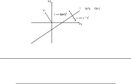
For fixed value z and c2 = 0, the objective function z = c1x1 + c2x2 is a straight line of the form
x2 = − c1 x1 + z , c2 c2
i.e. for different values of z we get parallel lines all with slope −c1/c2. The vector
c = |
c1 |
c2 |
points in the direction in which the objective function increases most. Thus, when maximizing the linear objective function z, we have to shift the line
x2 = − c1 x1 + z c2 c2
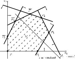
in the direction given by vector c, while when minimizing z, we have to shift this line in the opposite direction, given by vector −c. This is illustrated in Figure 9.1.
Based on the above considerations, an LPP of the form (9.7) with two variables can be graphically solved as follows:
(1)Determine the feasible region as the intersection of all feasible half-planes with the first quadrant. (This has already been discussed when describing the feasible region of a system of linear inequalities in Chapter 8.2.2.)
Linear programming 331
(2)Draw the objective function z = Z, where Z is constant, and shift it either in the direction given by vector c (in the case of z → max!) or in the direction given by vector −c (in the case of z → min!). Apply this procedure as long as the line z = constant has common
points with the feasible region.
Figure 9.1 The cases z → max! and z → min!
Example 9.2 A firm can manufacture two goods G1 and G2 in addition to its current production programme, where Table 9.2 gives the available machine capacities, the processing times for one unit of good Gi and the profit per unit of each good Gi, i {1, 2}.
Table 9.2 Data for Example 9.2
Process |
Processing times per unit |
Free machine capacity |
|
|
G1 |
G2 |
in minutes |
Turning |
0 |
8 |
640 |
Milling |
6 |
6 |
720 |
Planing |
6 |
3 |
600 |
Profit in EUR per unit |
1 |
2 |
— |
|
|
|
|
(1)First, we formulate the corresponding LPP. Let xi denote the number of produced units of good Gi, i {1, 2}. Then we obtain the following problem:
z = x1 + 2x2 → max!
s.t. |
+ |
8x2 |
≤ |
640 |
6x1 |
6x2 |
≤ |
720 |
|
6x1 |
+ |
3x2 |
≤ |
600 |
|
x1, x2 |
≥ |
0. |
|
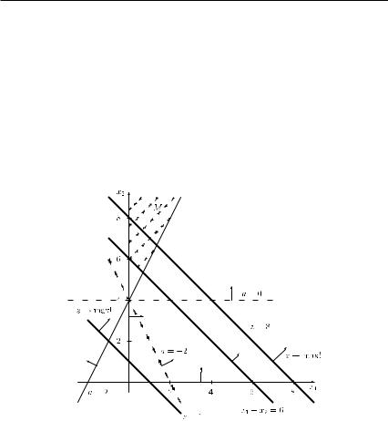
(2)We solve the above problem graphically (see Figure 9.2). We graph each of the three constraints as an equation and mark the corresponding half-spaces satisfying the given inequality constraint. The arrows on the constraints indicate the feasible half-space. The feasible region M is obtained as the intersection of these three feasible half-spaces
with the first quadrant. (We get the dashed area in Figure 9.2.) We graph the objective
function z = Z, where Z is constant. (In Figure 9.2 the parallel lines z = 0 and z = 200 are given.) The optimal extreme point is P4 corresponding to x1 = 40 and x2 = 80.
332 Linear programming
The optimal objective function value is z0max = x1 + 2x2 = 40 + 2 · 80 = 200. Notice that for z > 200, the resulting straight line would not have common points with the feasible region M .
Figure 9.2 Graphical solution of Example 9.2.
Next, we determine the basic feasible solutions corresponding to the extreme points P1, P2, . . . , P5. To this end, we introduce a slack variable in each constraint which yields the following system of constraints:
|
+ |
8x2 |
+ x3 |
= |
640 |
6x1 |
6x2 |
+ x4 |
= |
720 |
|
6x1 |
+ |
3x2 |
+x5 |
= |
600 |
|
|
|
x1, x2, x3, x4, x5 |
≥ 0. |
|
Considering point P1 with x1 = x2 = 0, the basic variables are x3, x4 and x5 (and consequently the matrix of the basis vectors is formed by the corresponding column vectors, which is an identity matrix). The values of the basic variables are therefore
x3 = 640, x4 = 720 and x5 = 600,
and the objective function value is z1 = 0. Considering point P2, we insert x1 = 100, x2 = 0 into the system of constraints, which yields the basic feasible solution
x1 = 100, x2 = 0, x3 = 640, x4 = 120, x5 = 0
with the objective function value z2 = 100. Considering point P3 with x1 = 80, x2 = 40, we obtain from the system of constraints the basic feasible solution
x1 = 80, x2 = 40, x3 = 320, x4 = 0, x5 = 0

334 Linear programming
It can be seen that all the resulting equations for different values of parameter a go through the point (0,4), and the slope of the line is given by 1/a for a = 0. To find the optimal solution, we now graph the objective function z = Z, where Z is constant. (In Figure 9.3 the lines z = 1 and z = 8 are shown.) The arrow on the lines z = constant indicates in which direction the objective function value increases. (Remember that the dashed area gives the feasible region M of the problem for a = 2.) From Figure 9.3, we see that the function value can become arbitrarily large (independently of the value of parameter a), i.e. an optimal solution of the maximization problem does not exist.
We continue with some properties of an LPP.
9.3PROPERTIES OF A LINEAR PROGRAMMING PROBLEM; STANDARD FORM
Let M be the feasible region and consider the maximization of the objective function z = cTx. We know already from Chapter 8.2.2 that the feasible region M of a system of linear inequalities is either empty or a convex polyhedron (see Theorem 8.10). Since the feasibility of a solution of an LPP is independent of the objective function, the latter property also holds for an LPP. We can further reinforce this and the following three cases for an LPP may occur:
(1)The feasible region is empty: M = . In this case the constraints are inconsistent, i.e. there is no feasible solution of the LPP.
(2)M is a non-empty bounded subset of the n-space Rn.
(3)M is an unbounded subset of the n-space Rn, i.e. at least one variable may become arbitrarily large, or if some variables are not necessarily non-negative, at least one of them may become arbitrarily small.
In case (2), the feasible region M is also called a convex polytope, and there is always a solution of the maximization problem. In case (3), there are again two possibilities:
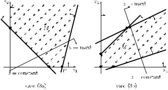
(3a) The objective function z is bounded from above. Then an optimal solution of the maximization problem under consideration exists.
(3b) The objective function z is not bounded from above. Then there does not exist an optimal solution for the maximization problem under consideration, i.e. there does not exist a finite optimal objective function value.
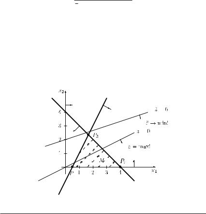
Cases (3a) and (3b) are illustrated in Figure 9.4. In case (3a), there are three extreme points, and P is an optimal extreme point. In case (3b), there exist four extreme points, however, the values of the objective function can become arbitrarily large.
Linear programming 335
Figure 9.4 The cases (3a) and (3b).
THEOREM 9.1 If an LPP has an optimal solution, then there exists at least one extreme point, where the objective function has an optimum value.
According to Theorem 9.1, one can restrict the search for an optimal solution to the consideration of extreme points (represented by basic feasible solutions). The following theorem characterizes the set of optimal solutions.
THEOREM 9.2 Let P1, P2, . . . , Pr described by vectors x1, x2, . . . , xr be optimal extreme points. Then any convex combination
|
r |
|
x0 = λ1x1 + λ2x2 + . . . + λr xr , λi ≥ 0, i = 1, 2, . . . , r, |
|
|
λi = 1 |
(9.8) |
i=1
is also an optimal solution.
PROOF Let x1, x2, . . . , xr be optimal extreme points with
cTx1 = cTx2 = . . . = cTxr = z0max
and x0 be defined as in (9.8). Then x0 is feasible since the feasible region M is convex. Moreover,
cTx0 = cT(λ1x1 + λ2x2 + . . . + λr xr ) = λ1(cTx1) + λ2(cTx2) + . . . + λr (cTxr ) |
|
= λ1z0max + λ2z0max + . . . + λr z0max = (λ1 + λ2 + . . . + λr )z0max = z0max, |
|
i.e. point x0 is optimal. |
|
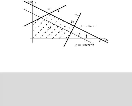
In Figure 9.5, Theorem 9.2 is illustrated for a problem with two variables having two optimal extreme points P1 and P2. Any point on the connecting line between the points P1 and P2 is optimal.
336 Linear programming
Figure 9.5 The case of several optimal solutions.
Standard form
In the next definition, we introduce a special form of an LPP.
Definition 9.2 An LPP of the form
z = cTx −→ max!
s.t. Ax = b, x ≥ 0,
where A = (AN , I ) and b ≥ 0 is called the standard form of an LPP.
According to Definition 9.2, matrix A can be partitioned into some matrix AN and an identity submatrix I . Thus, the standard form of an LPP is characterized by the following properties:
(1)the LPP is a maximization problem;
(2)the constraints are given as a system of linear equations in canonical form with nonnegative right-hand sides and
(3)all variables have to be non-negative.
It is worth noting that the standard form always includes a basic feasible solution for the corresponding system of linear inequalities (when the objective function is skipped). If no artificial variables are necessary when generating the standard form or when all artificial variables have value zero (this means that the right-hand sides of all constraints that contain an artificial variable are equal to zero), this solution is also feasible for the original problem and it corresponds to an extreme point of the feasible region M . However, it is an infeasible solution for the original problem if at least one artificial variable has a value greater than zero. In this case, the constraint from the original problem is violated and the basic solution does not correspond to an extreme point of set M . The generation of the standard form of an LPP plays an important role in finding a starting solution in the procedure that we present later for solving an LPP.
Any LPP can formally be transformed into the standard form by the following rules. We consider the possible violations of the standard form according to Definition 9.2.
Linear programming 337
(1)Some variable xj is not necessarily non-negative, i.e. xj may take arbitrary values. Then variable xj is replaced by the difference of two non-negative variables, i.e. we set:
xj = xj − xj with xj ≥ 0 and xj ≥ 0.
Then we get:
xj > xj xj > 0 xj = xj xj = 0 xj < xj xj < 0.
(2) The given objective function has to be minimized:
z = c1x1 + c2x2 + . . . + cnxn → min!
The determination of a minimum of function z is equivalent to the determination of a maximum of function z¯ = −z:
z = c1x1 + c2x2 + . . . + cnxn → min!
z¯ = −z = −c1x1 − c2x2 − . . . − cnxn → max!
(3) For some right-hand sides, we have bi < 0:
ai1x1 + ai2x2 + . . . + ainxn = bi < 0.
In this case, we multiply the above constraint by −1 and obtain:
−ai1x1 − ai2x2 − . . . − ainxn = −bi > 0.
(4) Let some constraints be inequalities:
ai1x1 + ai2x2 + . . . + ainxn ≤ bi
or
ak 1x1 + ak 2x2 + . . . + aknxn ≥ bk .
Then by introducing a slack variable ui and a surplus variable uk , respectively, we obtain an equation:
ai1x1 + ai2x2 + . . . + ainxn + ui = bi |
with |
ui ≥ 0 |
or |
|
|
ak 1x1 + ak 2x2 + . . . + aknxn − uk = bk |
with |
uk ≥ 0. |

338 Linear programming
(5)Let the given system of linear equations be not in canonical form, i.e. the constraints are given e.g. as follows:
a11x1 + a12x2 + . . . + a1nxn = b1 a21x1 + a22x2 + . . . + a2nxn = b2
.
.
.
am1x1 + am2x2 + . . . + amnxn = bm
with bi ≥ 0, i = 1, 2, . . . , m; xj ≥ 0, j = 1, 2, . . . , n.
In the above situation, there is no constraint that contains an eliminated variable with coefficient +1 (provided that all column vectors of matrix A belonging to variables x1, x2, . . . , xn are different from the unit vector). Then we introduce in each equation an artificial variable xAi as basic variable and obtain:
a11x1 + a12x2 + . . . + a1nxn + xA1 |
+ xA2 |
= b1 |
a21x1 + a22x2 + . . . + a2nxn |
= b2 |
|
. |
|
. |
. |
|
. |
. |
|
. |
am1x1 + am2x2 + . . . + amnxn |
|
+ xAm = bm |
with bi ≥ 0, i = 1, 2, . . . , m; xj ≥ 0, j = 1, 2, . . . , n, and xAi ≥ 0, i = 1, 2, . . . , m.
At the end, we may renumber the variables so that they are successively numbered. (For the above representation by x1, x2, . . . , xn+m, but in the following, we always assume that the problem includes n variables x1, x2, . . . , xn after renumbering.) In the way described above, we can transform any given LPP formally into the standard form. (It is worth noting again that a solution is only feasible for the original problem if all artificial variables have value zero.)
For illustrating the above transformation of an LPP into the standard form, we consider the following example.
Example 9.4 Given is the following LPP:
z = −x1 + 3x2 + x4 → min! |
− |
|
≥ |
|
||
s.t. x1 − x2 |
+ |
3x3 |
x4 |
8 |
||
x2 |
− |
5x3 |
+ 2x4 |
≤ −4 |
||
|
|
x3 |
+ |
x4 |
≤ |
3 |
|
|
|
x2, x3, x4 |
≥ |
0. |
|
First, we substitute for variable x1 the difference of two non-negative variables x1 and x1 , i.e. x1 = x1 − x1 with x1 ≥ 0 and x2 ≥ 0. Further, we multiply the objective function z by −1 and obtain:
|
= −z = x1 − x1 − 3x2 − x4 → max! |
|
|
|
|||||||
z |
|
|
|
||||||||
s.t. x |
− |
x |
− |
x2 |
+ |
3x3 |
− |
x4 |
≥ |
8 |
|
1 |
1 |
|
|
|
|
||||||
|
|
|
|
|
x2 |
− 5x3 |
+ 2x4 |
≤ −4 |
|||
|
|
|
|
|
|
|
x3 |
+ x4 |
≤ 3 |
||
|
|
|
|
|
|
x |
, x |
, x2, x3, x4 |
≥ |
0. |
|
|
|
|
|
|
|
1 |
1 |
|
|
|
|
Multiplying the second constraint by −1 and introducing the slack variable x7 in the third constraint as well as the surplus variables x5 and x6 in the first and second constraints, we

|
|
|
|
|
|
|
|
|
|
|
|
|
Linear programming |
339 |
|
obtain all constraints as equations with non-negative right-hand sides: |
|
|
|||||||||||||
|
|
= −z = x1 − x2 − 3x2 − x4 → max! |
|
|
|
|
|
|
|
|
|||||
|
z |
|
|
|
|
|
|
|
|
||||||
s.t. x |
x |
− |
x2 |
+ |
3x3 |
− |
x4 |
− |
x5 |
= |
8 |
||||
|
|
1 − |
1 |
|
|
|
|
− x6 |
|
||||||
|
|
|
|
− x2 |
+ 5x3 |
− 2x4 |
|
|
|
= 4 |
|||||
|
|
|
|
|
|
|
x3 |
+ |
x4 |
x |
, x |
+ x7 |
= |
3 |
|
|
|
|
|
|
|
|
|
|
|
, x2, x3, x4, x5, x6, x7 |
≥ |
0. |
|||
|
|
|
|
|
|
|
|
|
|
1 |
|
1 |
|
|
|
Now we can choose variable x1 as eliminated variable in the first constraint and variable x7 as the eliminated variable in the third constraint, but there is no variable that occurs only in the second constraint having coefficient +1. Therefore, we introduce the artificial variable xA1 in the second constraint and obtain:
|
|
= −z = x1 − x2 − 3x2 − x4 → max! |
|
|
|
||
|
z |
|
= 8 |
||||
s.t. − x1 − x2 + 3x3 |
− x4 |
− x5 + x1 |
+ xA1 |
||||
|
|
− x2 + 5x3 − 2x4 |
− x6 |
= 4 |
|||
|
|
x3 |
+ x4 |
|
+ x7 = 3 |
||
|
|
|
x , x , x2, x3, x4, x5, x6, x7, xA1 |
≥ |
0. |
||
|
|
|
1 |
1 |
|
|
|
Notice that we have written the variables in such a way that the identity submatrix (column vectors of variables x1 , xA1, x7) occurs at the end. So in the standard form, the problem has now n = 9 variables. A vector satisfying all constraints is only a feasible solution for the original problem if the artificial variable xA1 has value zero (otherwise the original second constraint would be violated).
9.4 SIMPLEX ALGORITHM
In this section, we always assume that the basic feasible solution resulting from the standard form of an LPP is feasible for the original problem. (In particular, we assume that no artificial variables are necessary to transform the given LPP into the standard form.) We now discuss a general method for solving linear programming problems, namely the simplex method. The basic idea of this approach is as follows. Starting with some initial extreme point (represented by a basic feasible solution resulting from the standard form of an LPP), we compute the value of the objective function and check whether the latter can be improved upon by moving to an adjacent extreme point (by applying the pivoting procedure). If so, we perform this move to the next extreme point and seek then whether further improvement is possible by a subsequent move. When finally an extreme point is attained that does not admit any further improvement, it will constitute an optimal solution. Thus, the simplex method is an iterative procedure which ends after a finite number of pivoting steps in an optimal extreme point (provided it is possible to move in each step to an adjacent extreme point). This idea is illustrated in Figure 9.6 for the case z → max! Starting from extreme point P1, one can go
via points P2 and P3 to the optimal extreme point P4 or via P2, P3, P4 to P4. In both cases, the objective function value increases from extreme point to extreme point.
In order to apply such an approach, a criterion to decide whether a move to an adjacent extreme point improves the objective function value is required, which we will derive in the following. We have already introduced the canonical form of a system of equations in Chapter 8.1.3 (see Definition 8.7). In the following, we assume that the rank of matrix A is equal to m, i.e. in the canonical form there are m basic variables among the n variables, and the number of non-basic variables is equal to n = n − m. Consider a feasible canonical form

Linear programming 341
Table 9.3 Simplex tableau of the basic feasible solution (9.9)
No. |
nbv |
xN 1 |
xN 2 |
· · · |
xNl |
· · · |
xNn |
|
|
bv |
-1 |
cN 1 |
cN 2 |
· · · |
cNl |
· · · |
cNn |
0 |
Q |
xB1 |
cB1 |
a |
a |
· · · |
a |
· · · |
a |
b |
|
xB2 |
cB2 |
11 |
12 |
1l |
1n |
|
1 |
||
a |
a |
· · · |
a |
· · · |
a |
b |
|||
. |
. |
. 21 |
. 22 |
. 2l |
. 2n |
. |
2 |
||
. |
. |
. |
. |
|
. |
|
. |
. |
|
. |
. |
. |
. |
|
. |
|
. |
. |
|
xBk |
cBk |
a |
a |
· · · |
a |
· · · |
a |
b |
|
. |
. |
. k1 |
. k2 |
. kl |
. kn |
. |
k |
||
. |
. |
. |
. |
|
. |
|
. |
. |
|
. |
. |
. |
. |
|
. |
|
. |
. |
|
xBm |
cBm |
a |
a |
· · · |
a |
· · · |
a |
b |
|
|
|
m1 |
m2 |
ml |
mn |
|
m |
||
z |
|
g1 |
g2 |
· · · |
gl |
· · · |
gn |
z0 |
|
Concerning the calculation of value z0 according to formula (9.11), we remember that in a basic solution, all non-basic variables are equal to zero.
Then we get the following representation of the objective function in dependence on the non-basic variables xNj :
z = z0 − g1xN 1 − g2xN 2 − . . . − gn xNn .
Here each coefficient gj gives the change in the objective function value if the non-basic variable xNj is included in the set of basic variables (replacing some other basic variable) and if its value would increase by one unit. By means of the coefficients in the objective row, we can give the following optimality criterion.
THEOREM 9.3 (optimality criterion) If inequalities gj ≥ 0, j = 1, 2, . . . , n , hold for the coefficients of the non-basic variables in the objective row, the corresponding basic feasible solution is optimal.
From Theorem 9.3 we get the following obvious corollary.
COROLLARY 9.1 If there exists a column l with gl < 0 in a basic feasible solution, the value of the objective function can be increased by including the column vector belonging to the non-basic variable xNl into the set of basis vectors, i.e. variable xNl becomes a basic variable in the subsequent basic feasible solution.
Assume that we have some current basic feasible solution (9.9). The corresponding simplex tableau is given in Table 9.3. It corresponds to the short form of the tableau of the pivoting procedure as introduced in Chapter 8.2.3 when solving systems of linear inequalities. An additional row contains the coefficients gj together with the objective function value z0 (i.e. the objective row) calculated as given above.
In the second row and column of the simplex tableau in Table 9.3, we write the coefficients of the corresponding variables in the objective function. Notice that the values of the objective row in the above tableau (i.e. the coefficients gj and the objective function value z0) are obtained as scalar products of the vector (−1, cB1, cB2, . . . , cBm)T of the second column
342 Linear programming
and the vector of the corresponding column (see formulas (9.10) and (9.11)). Therefore, numbers −1 and 0 in the second row are fixed in each tableau. In the left upper box, we write the number of the tableau. Note that the basic feasible solution (9.9) represented by Table 9.3 is not necessarily the initial basic feasible solution resulting from the standard form (in the latter case, we would simply have aij = aij and bi = bi for i = 1, 2, . . . , m and j = 1, 2, . . . , n provided that A = (aij ) is the matrix formed by the column vectors belonging to the initial non-basic variables).
If in the simplex tableau given in Table 9.3 at least one of the coefficients gj is negative, we have to perform a further pivoting step, i.e. we interchange one basic variable with a non-basic variable. This may be done as follows, where first the pivot column is determined, then the pivot row, and in this way the pivot element is obtained.
Determination of the pivot column l
Choose some column l, 1 ≤ l ≤ n , such that gl < 0. Often, a column l is used with
gl = min{gj | gj < 0, j = 1, 2, . . . , n }.
It is worth noting that the selection of the smallest negative coefficient gl does not guarantee that the algorithm terminates after the smallest possible number of iterations. It guarantees only that there is the biggest increase in the objective function value when going towards the resulting subsequent extreme point.
Determination of the pivot row k
We recall that after the pivoting step, the feasibility of the basic solution must be maintained. Therefore, we choose row k with 1 ≤ k ≤ m such that
b
= min i ail > 0, i = 1, 2, . . . , m .
It is the same selection rule which we have already used for the solution of systems of linear inequalities (see Chapter 8.2.3). To determine the above quotients, we have added the last column Q in the tableau given in Table 9.3, where we enter the quotient in each row in which the corresponding element in the chosen pivot column is positive.
If column l is chosen as pivot column, the corresponding variable xNl becomes a basic variable in the next step. We also say that xNl is the entering variable, and the column of the initial matrix A belonging to variable xNl is entering the basis. Using row k as pivot row, the corresponding variable xBk becomes a non-basic variable in the next step. In this case, we say that xBk is the leaving variable, and the column vector of matrix A belonging to variable xNl is leaving the basis. Element akl is known as the pivot or pivot element. It has been printed in bold face in the tableau together with the leaving and the entering variables.
The following two theorems characterize situations when either an optimal solution does not exist or when an existing optimal solution is not uniquely determined.
THEOREM 9.4 If inequality gl < 0 holds for a coefficient of a non-basic variable in the objective row and inequalities ail ≤ 0, i = 1, 2, . . . , m, hold for the coefficients in column l of the current tableau, then the LPP does not have an optimal solution.
Linear programming 343
In the latter case, the objective function value is unbounded from above, and we can stop our computations. Although there is a negative coefficient gl , we cannot move to an adjacent extreme point with a better objective function value (there is no leaving variable which can be interchanged with the non-basic variable xNl ).
THEOREM 9.5 If there exists a coefficient gl = 0 in the objective row of the tableau of an optimal basic feasible solution and inequality ail > 0 holds for at least one coefficient in column l, then there exists another optimal basic feasible solution, where xNl is a basic variable.
If the assumptions of Theorem 9.5 are satisfied, we can perform a further pivoting step with xNl as entering variable, and there is at least one basic variable which can be chosen as leaving variable. However, due to gl = 0, the objective function value does not change. Based on the results above, we can summarize the simplex algorithm as follows.
Simplex algorithm
(1)Transform the LPP into the standard form, where the constraints are given in canonical form as follows (remember that it is assumed that no artificial variables are necessary to transform the given problem into standard form):
AN xN + I xB = b, xN ≥ 0, xB ≥ 0, b ≥ 0,
where AN = (aij ) is of order m × n and b = (b1, b2, . . . , bm)T. The initial basic feasible solution is
x = |
xB |
= |
b |
|
xN |
|
0 |
with the objective function value z0 = cTx. Establish the corresponding initial tableau.
(2)Consider the coefficients gj , j = 1, 2, . . . , n , of the non-basic variables xNj in the
objective row.
If gj ≥ 0 for j = 1, 2, . . . , n , then the current basic feasible solution is optimal, stop. Otherwise, there is a coefficient gj < 0 in the objective row.
(3)Determine column l with
gl = min{gj | gj < 0, j = 1, 2, . . . , n }
as pivot column.
(4)If ail ≤ 0 for i = 1, 2, . . . , m, then stop. (In this case, there does not exist an optimal solution of the problem.) Otherwise, there is at least one element ail > 0.
(5)Determine the pivot row k such that
bk |
|
bi |
|
|
|
|
|
|
|
akl |
= min |
ail |
|
ail > 0, i = 1, 2, . . . , m . |
|
|
|
|
|
344 Linear programming
(6)Interchange the basic variable xBk of row k with the non-basic variable xNl of column l and calculate the following values of the new tableau:
akl |
1 |
|
|
|
|
|
|
|
|
|
||
= |
|
|
; |
|
|
|
|
|
|
|
|
|
akl |
|
|
|
|
|
|
|
|
||||
akj |
= |
akj |
|
|
bk = |
bk |
j = 1, 2, . . . , n , j = l; |
|||||
|
|
; |
|
|
|
; |
||||||
akl |
|
|
akl |
|||||||||
ail |
= − |
ail |
; |
i = 1, 2, . . . , m, i = k; |
||||||||
akl |
||||||||||||
aij |
|
|
|
|
|
ail |
|
|
|
bi = bi − |
ail |
|
= aij − |
|
· akj ; |
|
· bk ; |
||||||||
akl |
akl |
|||||||||||
|
|
|
|
i = 1, 2, . . . , m, |
i = k; j = 1, 2, . . . , n , j = l. |
|||||||
Moreover, calculate the values of the objective row in the new tableau:
gl = − |
gl |
; |
|
|
||
akl |
|
|
||||
gj = gj − |
|
gl |
|
· akj ; j = 1, 2, . . . , n , j = l; |
||
akl |
|
|||||
z0 = z0 − |
gl |
|
· bk . |
|||
akl |
|
|||||
Consider the tableau obtained as a new starting solution and go to step 2.
It is worth noting that the coefficients gj and the objective function value z0 in the objective row of new tableau can also be obtained by means of formulas (9.10) and (9.11), respectively, using the new values aij and bi .
If in each pivoting step the objective function value improves, the simplex method certainly terminates after a finite number of pivoting steps. However, it is possible that the objective function value does not change after a pivoting step. Assume that, when determining the pivot row, the minimal quotient is equal to zero. This means that some component of the current right-hand side vector is equal to zero. (This always happens when in the previous tableau the minimal quotient was not uniquely defined.) In this case, the basic variable xBk has the value zero, and in the next pivoting step, one non-basic variable becomes a basic variable again with value zero. Geometrically, this means that we do not move to an adjacent extreme point in this pivoting step: there is only one non-basic variable interchanged with some basic variable having value zero, and so it may happen that after a finite number of such pivoting steps with unchanged objective function value, we come again to a basic feasible solution that has already been visited. So, a cycle occurs and the procedure would not stop after a finite number of steps. We only mention that there exist several rules for selecting the pivot row and column which prevent such a cycling. One of these rules can be given as follows.
Smallest subscript rule. If there are several candidates for the entering and/or leaving variables, always choose the corresponding variables having the smallest subscript.
The above rule, which is due to Bland, means that among the non-basic variables with negative coefficient gj in the objective row, the variable with the smallest subscript is taken as the

Linear programming 345
entering variable and if, in this case, the same smallest quotient is obtained for several rows, then among the corresponding basic variables again the variable with the smallest subscript is chosen. However, since cycling occurs rather seldom in practice, the remote possibility of cycling is disregarded in most computer implementations of the simplex algorithm.
Example 9.5 Let us consider again the data given in Example 9.2. We can immediately give the tableau for the initial basic feasible solution:
1 |
nbv |
x1 |
x2 |
|
|
bv |
−1 |
1 |
2 |
0 |
Q |
x3 |
0 |
0 |
8 |
640 |
80 |
x4 |
0 |
6 |
6 |
720 |
120 |
x5 |
0 |
6 |
3 |
600 |
200 |
|
|
−1 |
−2 |
0 |
|
Choosing x2 as entering variable, we get the quotients given in the last column of the above tableau and thus we choose x3 as leaving variable. (Hereafter, both the entering and leaving variables are printed in bold face.) Number 8 (also printed in bold face) becomes the pivot element, and we get the following new tableau:
2 |
nbv |
x1 |
x3 |
|
|
bv |
−1 |
1 |
0 |
0 |
Q |
x2 |
2 |
0 |
1 |
80 |
— |
8 |
|||||
x4 |
0 |
6 |
− 43 |
240 |
40 |
x5 |
0 |
6 |
− 83 |
360 |
60 |
|
|
−1 |
1 |
160 |
|
|
|
4 |
|
Now, the entering variable x1 is uniquely determined, and from the quotient column we find x4 as the leaving variable. Then we obtain the following new tableau:
3 |
nbv |
x4 |
x3 |
|
|
|
bv |
−1 |
0 |
|
0 |
0 |
Q |
x2 |
2 |
0 |
|
1 |
80 |
|
|
8 |
|
||||
x1 |
1 |
1 |
− |
1 |
40 |
|
6 |
8 |
|
||||
x5 |
0 |
−1 |
|
3 |
120 |
|
|
8 |
|
||||
1 1 200
68
From the last tableau, we get the optimal solution which has already been found in Example 9.2 geometrically, i.e. the basic variables x1, x2 and x5 are equal to the corresponding values of the right-hand side: x1 = 40, x2 = 80, x5 = 120, and the non-basic variables x3 and x4 are equal to zero. We also see that the simplex method moves in each step

346 Linear programming
from an extreme point to an adjacent extreme point. Referring to Figure 9.2, the algorithm starts at point P1, moves then to point P5 and finally to the optimal extreme point P4. If in the first tableau variable x1 were chosen as the entering variable (which would also be allowed since the corresponding coefficient in the objective row is negative), the resulting path would be P1, P2, P3, P4, and in the latter case three pivoting steps would be necessary.
Example 9.6 A firm intends to manufacture three types of products P1, P2 and P3 so that the total production cost does not exceed 32,000 EUR. There are 420 working hours possible and 30 units of raw materials may be used. Additionally, the data presented in Table 9.4 are given.
Table 9.4 Data for Example 9.6
Product |
P1 |
P2 |
P3 |
Selling price (EUR/piece) |
1,600 |
3,000 |
5,200 |
Production cost (EUR/piece) |
1,000 |
2,000 |
4,000 |
Required raw material (per piece) |
3 |
2 |
2 |
Working time (hours per piece) |
20 |
10 |
20 |
|
|
|
|
The objective is to determine the quantities of each product so that the profit is maximized. Let xi be the number of produced pieces of Pi, i {1, 2, 3}. We can formulate the above problem as an LPP as follows:
z = 6x1 + 10x2 + 12x3 → max!
s.t. x1 |
+ |
2x2 |
+ |
4x3 |
≤ |
32 |
3x1 |
+ 2x2 |
+ 2x3 |
≤ 30 |
|||
2x1 |
+ |
x2 |
+ |
2x3 |
≤ 42 |
|
|
|
|
x1, x2, x3 |
≥ |
0. |
|
The objective function has been obtained by subtracting the production cost from the selling price and dividing the resulting profit by 100 for each product. Moreover, the constraint on the production cost has been divided by 1,000, and the constraint on the working time by 10.
Introducing now in the ith constraint the slack variable x3+i ≥ 0, we obtain the standard form together with the following initial tableau:
1 |
nbv |
x1 |
x2 |
x3 |
|
|
bv |
−1 |
6 |
10 |
12 |
0 |
Q |
x4 |
0 |
1 |
2 |
4 |
32 |
8 |
x5 |
0 |
3 |
2 |
2 |
30 |
15 |
x6 |
0 |
2 |
1 |
2 |
42 |
21 |
|
|
−6 |
−10 |
−12 |
0 |
|

Linear programming 347
Choosing x3 now as the entering variable (since it has the smallest negative coefficient in the objective row), variable x4 becomes the leaving variable due to the quotient rule. We obtain:
2 |
nbv |
x1 |
x2 |
x4 |
|
|
|
bv |
−1 |
6 |
10 |
|
0 |
0 |
Q |
x3 |
12 |
1 |
1 |
|
1 |
8 |
16 |
4 |
2 |
|
4 |
||||
x5 |
0 |
5 |
1 |
− |
1 |
14 |
14 |
2 |
2 |
||||||
x6 |
0 |
3 |
0 |
− |
1 |
26 |
− |
2 |
2 |
||||||
|
|
−3 |
−4 |
|
3 |
96 |
|
|
|
|
|
|
|
|
|
Choosing now x2 as entering variable, x5 becomes the leaving variable. We obtain the tableau:
3 |
nbv |
x1 |
x5 |
x4 |
|
|
||
bv |
−1 |
6 |
|
0 |
|
0 |
0 |
Q |
x3 |
12 |
−1 |
− |
1 |
|
1 |
1 |
|
2 |
|
2 |
|
|||||
x2 |
10 |
5 |
|
1 |
− |
1 |
14 |
|
2 |
|
2 |
|
|||||
x6 |
0 |
3 |
|
0 |
− |
1 |
26 |
|
2 |
|
2 |
|
|||||
|
|
7 |
|
4 |
|
1 |
152 |
|
|
|
|
|
|
|
|
|
|
Since now all coefficients gj are positive, we get the following optimal solution from the latter tableau:
x1 = 0, x2 = 14, x3 = 1, x4 = 0, x5 = 0, x6 = 26.
This means that the optimal solution is to produce no piece of product P1, 14 pieces of product P2 and one piece of product P3. Taking into account that the coefficients of the objective function were divided by 100, we get a total profit of 15,200 EUR.
Example 9.7 We consider the following LPP:
z = −2x1 − 2x2 → min! |
−1 |
|||
s.t. x1 |
− |
x2 |
≥ |
|
−x1 |
+ |
2x2 |
≤ |
4 |
|
x1, x2 |
≥ |
0. |
|
First, we transform the given problem into the standard form, i.e. we multiply the objective function and the first constraint by −1 and introduce the slack variables x3 and x4. We obtain:
z = 2x1 + 2x2 → max!
s.t. − x1 |
+ |
x2 |
+ x3 |
= |
1 |
− x1 |
+ |
2x2 |
+ x4 |
= 4 |
|
|
|
|
x1, x2, x3, x4 |
≥ |
0. |

348 Linear programming
Now we can establish the first tableau:
1 |
nbv |
x1 |
x2 |
|
|
bv |
−1 |
2 |
2 |
0 |
Q |
x3 |
0 |
−1 |
1 |
1 |
1 |
x4 |
0 |
−1 |
2 |
4 |
2 |
|
|
−2 |
−2 |
0 |
|
Since there are only negative elements in the column of variable x1, only variable x2 can be the entering variable. In this case, we get the quotients given in the last column of the latter tableau and therefore, variable x3 is the leaving variable. We obtain the following tableau:
2 |
nbv |
x1 |
x3 |
|
|
bv |
−1 |
2 |
0 |
0 |
Q |
x2 |
2 |
−1 |
1 |
1 |
– |
x4 |
0 |
1 |
−2 |
2 |
2 |
|
|
−4 |
2 |
2 |
|
In the latter tableau, there is only one negative coefficient of a non-basic variable in the objective row, therefore variable x1 becomes the entering variable. Since there is only one positive element in the column belonging to x1, variable x4 becomes the leaving variable. We obtain the following tableau:
3 |
nbv |
x4 |
x3 |
|
|
bv |
−1 |
0 |
0 |
0 |
Q |
x2 |
2 |
1 |
−1 |
3 |
|
x1 |
2 |
1 |
−2 |
2 |
|
|
|
4 |
−6 |
10 |
|
Since there is only one negative coefficient of a non-basic variable in the objective row, variable x3 should be chosen as entering variable. However, there are only negative elements in the column belonging to x3. This means that we cannot perform a further pivoting step, and so there does not exist an optimal solution of the maximization problem considered (i.e. the objective function value can become arbitrarily large, see Theorem 9.4).
Example 9.8 Given is the following LPP:
z = x1 + x2 + x3 + x4 + x5 + x6 → min!
s.t. 2x1 + x2 |
+ x3 |
+ 2x4 + x5 |
≥ 4, 000 |
|
x2 |
|
≥ 5, |
000 |
|
|
x3 |
+ 2x5 |
+ 3x6 ≥ 3, |
000 |
x1, x2, x3, x4, x5, x6 ≥ 0.
To get the standard form, we notice that in each constraint there is one variable that occurs only in this constraint. (Variable x1 occurs only in the first constraint, variable x4 only in the second constraint and variable x6 only in the third constraint.) Therefore, we divide the first constraint by the coefficient 2 of variable x1, the second constraint by 2 and the third

Linear programming 349
constraint by 3. Then, we introduce a surplus variable in each of the constraints, multiply the objective function by −1 and obtain the standard form. (Again the variables are written in such a way that the identity submatrix of the coefficient matrix occurs now at the end.)
|
= −z |
1= −x11− x2 − x3 − x4 − x5 − x6 → max! |
||||
z |
||||||
s.t. |
2 x2 + 2 x3 |
+ 21 x5 |
− x7 |
+ x1 |
= 2, 000 |
|
|
|
21 x2 |
|
− x8 |
+ x4 = 2, 500 |
|
|
|
31 x3 |
+ 32 x5 |
|
− x9 |
+ x6 = 1, 000 |
|
|
|
|
x1, x2, x3, x4, x5, x6, x7, x8, x9 ≥ 0. |
||
This yields the following initial tableau:
1 |
nbv |
x2 |
x3 |
x5 |
x7 |
x8 |
x9 |
|
|
|
bv −1 |
−1 −1 −1 |
0 |
0 |
0 |
0 |
Q |
||||
x1 |
−1 |
1 |
1 |
|
0 |
−1 |
0 |
0 |
2,000 |
− |
2 |
2 |
|
||||||||
x4 |
−1 |
1 |
0 |
|
1 |
0 |
−1 |
0 |
2,500 |
5,000 |
2 |
|
2 |
||||||||
x6 |
−1 |
0 |
1 |
|
2 |
0 |
0 |
−1 |
1,000 |
1,500 |
3 |
|
3 |
||||||||
|
|
|||||||||
|
|
0 |
1 |
− |
1 |
1 |
1 |
1 |
− 5,500 |
|
|
|
6 |
6 |
|
||||||
Choosing now x5 as entering variable, we obtain the quotients given in the last column of the above tableau and therefore, x6 is chosen as leaving variable. We obtain the following tableau:
2 |
nbv |
x2 |
x3 |
x6 |
x7 |
x8 |
x9 |
|
|
|||
bv −1 |
−1 −1 −1 |
0 |
0 |
|
0 |
0 |
Q |
|||||
x1 |
−1 |
1 |
|
1 |
|
0 |
−1 |
0 |
|
0 |
2,000 |
|
2 |
|
2 |
|
|
|
|||||||
x4 |
−1 |
1 |
− |
1 |
− |
3 |
0 |
−1 |
|
3 |
1,750 |
|
2 |
4 |
4 |
|
4 |
|
|||||||
x5 |
−1 |
0 |
|
1 |
|
3 |
0 |
0 |
− |
3 |
1,500 |
|
|
2 |
|
2 |
2 |
|
|||||||
|
|
0 |
|
1 |
|
1 |
1 |
1 |
|
3 |
−5,250 |
|
|
|
|
4 |
|
4 |
|
4 |
|
||||
Now all coefficients of the non-basic variables in the objective row are non-negative and from the latter tableau we obtain the following optimal solution:
x1 = 2, 000, x2 = x3 = 0, x4 = 1, 750, x5 = 1, 500, x6 = 0
with the optimal objective function value zmax0 = −5, 250 which corresponds to z0min = 5, 250 (for the original minimization problem). Notice that the optimal solution is not uniquely determined. In the last tableau, there is one coefficient in the objective row equal to zero. Taking x2 as the entering variable, the quotient rule determines x4 as the leaving variable, and the following basic feasible solution with the same objective function value is obtained:
x1 = 250, x2 = 3, 500, x3 = x4 = 0, x5 = 1, 500, x6 = 0.
350 Linear programming
9.5 TWO-PHASE SIMPLEX ALGORITHM
In this section, we discuss the case when artificial variables are necessary to transform a given problem into standard form. In such a case, we have to determine a basic solution feasible for the original problem that can also be done by applying the simplex algorithm. This procedure is called phase I of the simplex algorithm. It either constructs an initial basic feasible solution or recognizes that the given LPP does not have a feasible solution at all. If a feasible starting solution has been found, phase II of the simplex algorithm starts, which corresponds to the simplex algorithm described in Chapter 9.4.
The introduction of artificial variables is necessary when at least one constraint is an equation with no eliminated variable that has coefficient +1, e.g. the constraints may have the following form:
a11 x1 + a12x2 + · · · + a1nxn = b1 a21 x1 + a22x2 + · · · + a2nxn = b2
. |
. |
. |
. |
. |
. |
am1x1 + am2x2 + · · · + amnxn = bm |
|
xj ≥ 0, j = 1, 2, . . . , n; |
bi ≥ 0, i = 1, 2, . . . , m. |
As discussed in step (5) of generating the standard form, we introduce an artificial variable xAi in each equation. Additionally we replace the original objective function z by an objective function zI minimizing the sum of all artificial variables (or equivalently, maximizing the negative sum of all artificial variables) since it is our goal that all artificial variables will get value zero to ensure feasibility for the original problem. This gives the following linear programming problem to be considered in phase I:
zI = −xA1 − xA2 − . . . − xAm −→ max!
s.t. a11 x1 + a12x2 + . . . + a1nxn + xA1 |
+ xA2 |
= b1 |
|
a21 x1 + a22x2 + . . . + a2nxn |
= b2 |
(9.12) |
|
. |
|
. |
|
. |
|
. |
|
. |
|
. |
|
am1x1 + am2x2 + . . . + amnxn |
|
+ xAm = bm |
|
xj ≥ 0, j = 1, 2, . . . , n and xAi |
≥ 0, i = 1, 2, . . . , m. |
|
|
The above problem is the standard form of an LPP with function z replaced by function zI . The objective function zI used in the first phase is also called the auxiliary objective function. When minimizing function zI , the smallest possible objective function value is equal to zero. It is attained when all artificial variables have value zero, i.e. the artificial variables have become non-basic variables, or possibly some artificial variable is still a basic variable but it has value zero. When an artificial variable becomes the leaving variable (and therefore has value zero in the next tableau), it never will be the entering variable again, and therefore this variable together with the corresponding column can be dropped in the new tableau.

352 Linear programming
Choosing x1 as entering variable gives the quotients presented in the last column of the above tableau, and variable xA1 becomes the leaving variable. This leads to the following tableau:
2 |
nbv |
xA1 |
x2 |
x3 |
|
|||
bv |
−1 |
−1 |
|
0 |
|
0 |
0 Q |
|
x4 |
0 |
− |
1 |
|
3 |
|
1 |
7 |
2 |
|
2 |
|
2 |
2 |
|||
x1 |
0 |
|
1 |
− |
1 |
− |
1 |
1 |
|
2 |
2 |
2 |
2 |
||||
|
|
|
1 |
|
0 |
|
0 |
0 |
|
|
|
|
|
|
|
|
|
Now phase I is finished, we drop variable xA1 and the corresponding column, use the original objective function and determine the coefficients gj of the objective row. This yields the following tableau:
2 |
nbv |
x2 |
x3 |
|
|
||
bv |
−1 |
−2 |
|
0 |
0 |
Q |
|
x4 |
0 |
|
3 |
|
1 |
7 |
7 |
|
2 |
|
2 |
2 |
|||
x1 |
1 |
− |
1 |
− |
1 |
1 |
− |
2 |
2 |
2 |
|||||
|
|
|
3 |
− |
1 |
1 |
|
|
|
|
2 |
2 |
2 |
|
|
Due to the negative coefficient in the objective row, we choose x3 as the entering variable in the next step and variable x4 becomes the leaving variable. Then we obtain the following tableau
3 |
nbv |
x2 |
x4 |
|
|
bv |
−1 |
−2 |
0 |
0 |
Q |
x3 |
0 |
3 |
2 |
7 |
|
x1 |
1 |
1 |
1 |
4 |
|
|
|
3 |
1 |
4 |
|
|
|
|
|
|
|
Since all coefficients gj are non-negative, the obtained solution is optimal: x1 = 4, x2 = 0. The introduced surplus variable x3 is equal to seven while the introduced slack variable x4 is equal to zero. The optimal objective function value is z0max = 4. The graphical solution of this problem is illustrated in Figure 9.7. We see from Figure 9.7 that the origin of the coordinate system with variables x1 and x2 is not feasible since the second constraint is violated. This was the reason for introducing the artificial variable xA1 which has initially the value one. After the first pivoting step, we get a feasible solution for the original problem which corresponds to extreme point P1 in Figure 9.7. Now phase II of the simplex algorithm starts, and after the next pivoting step we reach an adjacent extreme point P2 which corresponds to an optimal solution of the considered LPP.
Let us consider another LPP assuming that the objective function changes now to
z˜ = −x1 + 3x2 −→ min!
Linear programming 353
Can we easily decide whether the optimal solution for the former objective function is also optimal for the new one? We replace only the coefficients c1 and c2 of the objective function in the last tableau (again for the maximization version of the problem), recompute the coefficients gj of the objective row and obtain the following tableau:
3 |
nbv |
x2 |
x4 |
|
|
bv |
−1 |
−3 |
0 |
0 |
Q |
x3 |
0 |
3 |
2 |
7 |
|
x1 |
1 |
1 |
1 |
4 |
|
|
|
4 |
1 |
4 |
|
|
|
|
|
|
|
Since also in this case all coefficients gj in the objective row are non-negative, the solution x1 = 4, x2 = 0 is optimal for z˜ = −x1 + 3x2 −→ min as well with a function value z˜0min = −4. This can also be confirmed by drawing the objective function z˜ in Figure 9.7.
Figure 9.7 Graphical solution of Example 9.9.
Example 9.10 We consider the data given in Example 9.1 and apply the two-phase simplex method. Transforming the given problem into standard form we obtain:
|
= −25x1 − 17x2 − 12x3 → max! |
|
|
||||
z |
= |
|
|||||
s.t. x1 |
+ x2 |
+ |
x3 |
+ xA1 |
100 |
||
|
|
|
+ |
x3 |
+ x4 |
= |
30 |
|
x1 |
|
x3 |
+ x5 |
= |
50 |
|
|
|
x2 |
+ |
x3 |
+ x6 |
= |
90 |
|
|
|
|
|
x1, x2, x3, x4, x5, x6, xA1 |
≥ 0. |
|

354 Linear programming
Starting with phase I of the simplex method, we replace function z by the auxiliary objective function
zI = −xA1 −→ max!
We obtain the following initial tableau:
1 |
nbv |
x1 |
x2 |
x3 |
|
|
bv |
−1 |
0 |
0 |
0 |
0 |
Q |
xA1 |
−1 |
1 |
1 |
1 |
100 |
100 |
x4 |
0 |
0 |
0 |
1 |
30 |
− |
x5 |
0 |
1 |
0 |
1 |
50 |
50 |
x6 |
0 |
0 |
1 |
1 |
90 |
− |
|
|
−1 |
−1 |
−1 |
−100 |
|
Choosing x1 as the entering variable, we get the quotients given above and select x5 as the leaving variable. This leads to the following tableau:
2 |
nbv |
x5 |
x2 |
x3 |
|
|
bv |
−1 |
0 |
0 |
0 |
0 |
Q |
xA1 |
−1 |
−1 |
1 |
0 |
50 |
50 |
x4 |
0 |
0 |
0 |
1 |
30 |
− |
x1 |
0 |
1 |
0 |
1 |
50 |
− |
x6 |
0 |
0 |
1 |
1 |
90 |
90 |
|
|
1 |
−1 |
0 |
− 50 |
|
Now x2 becomes the entering variable and the artificial variable xA1 is the leaving variable. We get the following tableau, where the superfluous column belonging to xA1 is dropped.
3 |
nbv |
x5 |
x3 |
|
|
bv |
−1 |
0 |
0 |
0 |
Q |
x2 |
0 |
−1 |
0 |
50 |
|
x4 |
0 |
0 |
1 |
30 |
|
x1 |
0 |
1 |
1 |
50 |
|
x6 |
0 |
1 |
1 |
40 |
|
|
|
0 |
0 |
0 |
|
|
|
|
|
|
|
Now, phase I is finished, and we can consider the objective function
z = −25x1 − 17x2 − 12x3 −→ max!

Linear programming 355
We recompute the coefficients in the objective row and obtain the following tableau:
3 |
nbv |
x5 |
x3 |
|
|
bv |
−1 |
0 |
−12 |
0 |
Q |
x2 |
−17 |
−1 |
0 |
50 |
− |
x4 |
0 |
0 |
1 |
30 |
30 |
x1 |
−25 |
1 |
1 |
50 |
50 |
x6 |
0 |
1 |
1 |
40 |
40 |
|
|
−8 |
−13 |
−2,100 |
|
We choose x3 as entering variable and based on the quotients given in the last column, x4 is the leaving variable. After this pivoting step, we get the following tableau:
4 |
nbv |
x5 |
x4 |
|
|
bv |
−1 |
0 |
0 |
0 |
Q |
x2 |
−17 |
−1 |
0 |
50 |
− |
x3 |
−12 |
0 |
1 |
30 |
− |
x1 |
−25 |
1 |
−1 |
20 |
20 |
x6 |
0 |
1 |
−1 |
10 |
10 |
|
|
−8 |
13 |
−1,710 |
|
We choose x5 as entering variable and x6 as leaving variable which gives the following tableau:
5 |
nbv |
x6 |
x4 |
|
|
bv |
−1 |
0 |
0 |
0 |
Q |
x2 |
−17 |
1 |
−1 |
60 |
|
x3 |
−12 |
0 |
1 |
30 |
|
x1 |
−25 |
−1 |
0 |
10 |
|
x5 |
0 |
1 |
−1 |
10 |
|
|
|
8 |
5 |
−1,630 |
|
This last tableau gives the following optimal solution:
x1 = 10, x2 = 60, x3 = 30, x4 = 0, x5 = 10, x6 = 0
with the objective function value z0min = 1, 630 for the minimization problem.
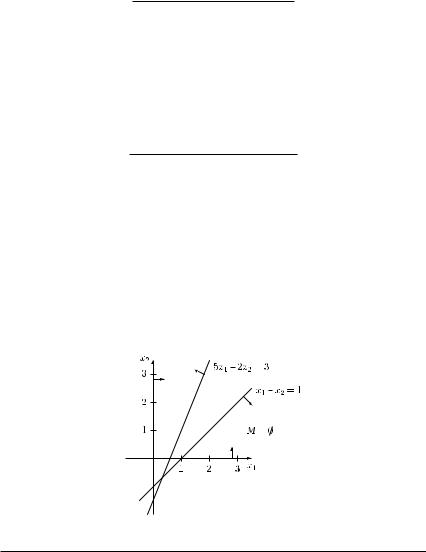
Example 9.11 Consider the following LPP:
z = x1 + 2x2 → max!
s.t. x1 |
− |
x2 |
≥ |
1 |
5x1 |
− |
2x2 |
≤ |
3 |
|
x1, x2 |
≥ |
0. |
|

Linear programming 357
Remark For many problems, it is possible to reduce the number of artificial variables to be considered in phase I. This is important since in any pivoting step, only one artificial variable is removed from the set of basic variables. Thus, in the case of introducing m artificial variables, at least m pivoting steps are required in phase I. Let us consider the following example.
Example 9.12 Consider the following constraints of an LPP:
−2x1 |
|
2x2 |
− |
x3 |
− x4 |
+ x5 |
≥ 1 |
|
− |
|
+ 2x3 |
− x4 |
+ |
x5 |
≥ 2 |
||
x1 |
2x2 |
+ |
|
− x4 |
+ |
x5 |
≥ 3 |
|
x1 |
+ |
x2 |
x3 |
|
|
|
≥ 5 |
|
|
|
|
|
|
x1, x2, x3, x4, x5 |
≥ 0. |
||
First, we introduce in each constraint a surplus variable and obtain
2x2 − x3 − x4 + x5 − x6 |
− x7 |
= 1 |
|
−2x1 |
+ 2x3 − x4 + x5 |
= 2 |
|
x1 − 2x2 |
− x4 + x5 |
|
− x8 = 3 |
x1 + x2 + x3 |
|
− x9 = 5 |
|
|
x1, x2, x3, x4, x5, x6, x7, x8, x9 ≥ 0. |
||
Now, we still need an eliminated variable with coefficient +1 in each equation constraint. Instead of introducing an artificial variable in each of the constraints, we subtract all other constraints from the constraint with the largest right-hand side. In this example, we get the first three equivalent constraints by subtracting the corresponding constraint from the fourth constraint:
x1 |
− x2 |
+ 2x3 |
+ x4 |
− x5 |
− x9 |
+ x6 |
= 4 |
||||||
3x1 |
+ |
x2 |
− x3 |
+ |
x4 |
− |
x5 |
− x9 |
+ x7 |
= 3 |
|||
|
+ |
3x2 |
+ |
x3 |
+ |
x4 |
− |
x5 |
− |
x9 |
|
+ x8 = |
2 |
x1 |
x2 |
+ |
x3 |
|
|
|
|
− |
x9 |
|
= |
5 |
|
x1, x2, x3, x4, x5, x6, x7, x8, x9 ≥ 0.
Now we have to introduce only one artificial variable xA1 in the last constraint in order to start with phase I of the simplex algorithm.
9.6 DUALITY; COMPLEMENTARY SLACKNESS
We consider the following LPP denoted now as primal problem (P):
z = cTx −→ max! |
|
s.t. Ax ≤ b |
(P) |
x ≥ 0, |
|

358 Linear programming
where x = (x1, x2, . . . , xn)T Rn. By means of matrix A and vectors c and b, we can define a dual problem (D) as follows:
w = bTu −→ min! |
|
T |
|
s.t. A u ≥ c |
(D) |
u ≥ 0, |
|
where u = (un+1, un+2, . . . , un+m)T Rm. Thus, the dual problem (D) is obtained by the following rules:
(1)The coefficient matrix A of problem (P) is transposed.
(2)The variables of the dual problem are denoted as un+1, un+2, . . . , un+m, and they have to be non-negative.
(3)The vector b of the right-hand side of problem (P) is the vector of the objective function of problem (D).
(4)The vector c of the objective function of the primal problem (P) is the vector of the right-hand side of the dual problem (D).
(5)In all constraints of the dual problem (D), we have inequalities with the relation ≥.
(6)The objective function of the dual problem (D) has to be minimized.
By ‘dualizing’ problem (P), there is an assignment between the constraints of the primal problem (P) and the variables of the dual problem (D), and conversely, between the variables of problem (P) and the constraints of problem (D). Both problems can be described by the scheme given in Table 9.5 which has to be read row-wise for problem (P) and column-wise for problem (D).
Table 9.5 Relationships between problems (P) and (D)
|
x1 |
x2 |
. . . |
xn |
≤ |
|
|
un+1 |
a11 |
a12 |
. . . |
a1n |
b1 |
|
|
u |
a |
a |
. . . |
a |
b |
|
|
. n+2 |
. 21 |
. 22 |
|
. 2n |
. 2 |
|
|
. |
. |
. |
|
. |
. |
|
|
. |
. |
. |
|
. |
. |
|
|
un+m |
am1 |
am2 |
. . . |
amn |
bm |
|
|
≥ |
c1 |
c2 |
|
cn |
min! |
|
|
. . . |
max! |
|
|||||
|
|
|
|
|
|
|
|
For instance, the first constraint of problem (P) reads as
a11x1 + a12x2 + . . . + a1nxn ≤ b1
while e.g. the second constraint of problem (D) reads as
a12un+1 + a22un+2 + . . . + am2un+m ≥ c2.
Notice that the variables are successively numbered, i.e. the n variables of the primal problem
(P) are indexed by 1, 2, . . . , n while the m variables of the dual problem (D) are indexed by n + 1, n + 2, . . . , n + m. We get the following relationships between problems (P) and (D).
THEOREM 9.6 Let problem (D) be the dual problem of problem (P). Then the dual problem of problem (D) is problem (P).

360 Linear programming
are equal to the coefficients of the corresponding dual variables in the objective row of the optimal tableau of problem (P).
Thus, from the optimal tableau of one of the problems (P) or (D), we can determine the optimal solution of the other one.
Example 9.13 Consider the data given in Example 9.2. The optimal tableau for this problem has been determined in Example 9.5. Writing the dual problem with the constraints as in (D ), we obtain:
w = 640u3 + 720u4 + 600u5 −→ min! |
+ |
|
= 1 |
||
s.t. − u1 |
+ |
6u4 |
6u5 |
||
− u2 |
+ 8u3 + |
6u4 |
+ |
3u5 |
= 2 |
|
u1, u2, u3, u4, u5 |
≥ 0. |
|||
Applying Theorem 9.10, we get the following. Since in the optimal solution given in Example 9.5, variables x4 and x3 are non-basic variables, the corresponding variables u4 and u3 are basic variables in the optimal solution of the dual problem and their values are equal to the coefficients of x4 and x3 in the objective row of the optimal tableau of the primal problem, i.e. u4 = 1/6 and u3 = 1/8. Since x2, x1 and x5 are basic variables in the optimal tableau of the primal problem, the variables u2, u1 and u5 are non-basic variables in the optimal solution of the dual problem, i.e. their values are equal to zero. Accordingly, the values of the right-hand side in the optimal primal tableau correspond to the coefficients of the dual non-basic variables in the objective row, i.e. they are equal to 80, 40 and 120, respectively.
Finally, we briefly deal with a ‘mixed’ LPP (i.e. equations may occur as constraints, we may have inequalities both with ≤ and ≥ sign, and variables are not necessarily non-negative). Then we can establish a dual problem using the rules given in Table 9.6. To illustrate, let us consider the following example.
Example 9.14 Consider the LPP
z = 2x1 + 3x2 + 4x3 −→ max! |
≤ |
|
||
s.t. x1 |
− x2 |
+ x3 |
20 |
|
−3x1 |
+ x2 |
+ x3 |
≥ 3 |
|
4x1 |
− x2 |
+ 2x3 |
= 10 |
|
x1 ≥ 0 |
|
x3 |
≤ |
5 |
(x2, x3 arbitrary). |
|
|||
Applying the rules given in Table 9.6, we obtain the following dual problem:
w = 20u4 + 3u5 + 10u6 + 5u7 −→ min!
s.t. u4 |
− 3u5 |
+ |
4u6 |
≥ 2 |
|
−u4 |
+ |
u5 |
− u6 |
= 3 |
|
u4 |
+ |
u5 |
+ |
2u6 |
+ u7 = 4 |
u4 ≥ 0, u5 ≤ 0, u7 ≥ 0 |
(u6 arbitrary). |
||||
|
|
|
|
|
|

|
|
Linear programming 361 |
|
Table 9.6 Rules for dualizing a problem |
|
|
|
|
|
|
|
Primal problem |
|
Dual problem |
|
(P) |
|
(D) |
|
Maximization problem |
|
Minimization problem |
|
Constraints |
= |
Variables |
|
ith constraint: inequality with sign ≤ |
un+i ≥ 0 |
||
ith constraint: inequality with sign ≥ |
= |
un+i ≤ 0 |
|
ith constraint: equation |
= |
un+i arbitrary |
|
Variables |
= |
Constraints |
|
xj ≥ 0 |
jth constraint: inequality with sign ≥ |
||
xj ≤ 0 |
= |
jth constraint: inequality with sign ≤ |
|
xj arbitrary |
= |
jth constraint: equation |
|
We finish this section with an economic interpretation of duality. Consider problem (P) as the problem of determining the optimal production quantities xj of product Pj , j = 1, 2, . . . , n, subject to given budget constraints, i.e. for the production there are m raw materials required and the right-hand side value bi gives the available quantity of raw material Ri, i {1, 2, . . . , m}. The objective is to maximize the profit described by the linear function cTx. What is the economic meaning of the corresponding dual variables of problem
(D) in this case? Assume that we increase the available amount of raw material Ri by one unit (i.e. we use the right-hand side component bi = bi + 1) and all other values remain constant. Moreover, assume that there is an optimal non-degenerate basic solution (i.e. all basic variables have a value greater than zero) and that the same basic solution is optimal for the modified problem (P ) with bi replaced by bi (i.e. no further pivoting step is required). In this case, the optimal function value zmax0 of problem (P ) is given by
zmax0 = b1un+1 + . . . + (bi + 1)un+i + . . . + bmun+m = w0min + un+i,
where u = (un+1, un+2, . . . , un+m)T denotes the optimal solution of the dual problem (D). The latter equality holds due to Theorem 9.8 (i.e. z0max = w0min). This means that after ‘buying’ an additional unit of resource Ri, the optimal function value increases by the value un+i. Hence, the optimal values un+i of the variables of the dual problem can be interpreted as shadow prices for buying an additional unit of raw materials Ri, i.e. un+i characterizes the price that a company is willing to pay for an additional unit of raw material Ri, i = 1, 2, . . . , m.
Next, we consider the primal problem (P) and the dual problem (D). We can formulate the following relationship between the optimal solutions of both problems.
THEOREM 9.11 Let x = (x1 , x2 , . . . , xn )T be a feasible solution of problem (P) and u = (un+1, un+2, . . . , un+m)T be a feasible solution of problem (D). Then both solutions x and u are simultaneously optimal if and only if the following two conditions hold:
|
m |
|
|
|
|
|
|
|
|
(1) |
n |
= |
j |
= |
0 for j |
= |
1, 2, . . . , n; |
||
n+i |
|||||||||
aij u |
|
cj or x |
|
|
|
||||
|
i=1 |
|
|
|
|
|
|
|
|
|
|
|
n+i |
= |
|
|
= |
|
|
(2) |
j = |
bi |
0 for i |
1, 2, . . . , m. |
|||||
aij x |
or u |
|
|
|
|||||
j=1
362 Linear programming
Theorem 9.11 means that vectors x and u are optimal for problems (P) and (D) if and only if
(1)either the jth constraint in problem (D) is satisfied with equality or the jth variable of problem (P) is equal to zero (or both) and
(2)either the ith constraint in problem (P) is satisfied with equality or the ith variable of problem (D) (i.e. un+i = 0) is equal to zero (or both).
Theorem 9.11 can be rewritten in the following form:
THEOREM 9.12 A feasible solution x = (x1 , x2 , . . . , xn )T of problem (P) is optimal if and only if there exists a vector u = (un+1, un+2, . . . , un+m)T such that the following two properties are satisfied:
|
|
n |
|
m |
|
|
|
|
(1) |
|
|
|
aij u |
|
cj ; |
|
|
if x |
> 0, then |
= |
(9.13) |
|||||
|
|
j |
|
i=1 |
n+i |
|
||
|
|
aij xj |
|
|
|
|
||
(2) |
if |
< bi, |
then un+i |
= 0, |
|
|||
j=1
provided that vector u is feasible for problem (D), i.e.
m |
|
|
|
|
|
|
|
|
|
u |
≥ |
c |
|
for j |
= |
1, 2, . . . , n; |
|
a |
j |
|||||||
ij |
|
n+i |
|
|
(9.14) |
|||
i=1 |
|
|
|
|
|
|
= |
|
n+i ≥ |
0 |
|
|
|
for i |
1, 2, . . . , m. |
||
u |
|
|
|
|
|
|||
Remark Theorem 9.12 is often useful in checking the optimality of allegedly optimal solutions when no certificate of optimality is provided. Confronted with an allegedly optimal solu-
tion x of problem (P), we first set up the system of linear equations (9.13) and solve it for u =
(un+1, un+2, . . . , un+m)T. If the solution u = (un+1, un+2, . . . , un+m)T is uniquely determined, then vector x is optimal if and only if vector u is feasible, i.e. conditions (9.14) hold.
Example 9.15 Consider the LPP in Example 9.2 and the corresponding dual problem established in Example 9.13. Assume that we still do not know an optimal solution, but we want to use complementary slackness to verify that x1 = 40, x2 = 80 is indeed an optimal solution for problem (P). It follows from the second condition of (9.13) that u5 = 0 since, for the third constraint of the primal problem, we have
6x1 + 3x2 = 6 · 40 + 3 · 80 = 480 < 600
while the other two constraints of the primal problem are satisfied with equality, i.e.
8x2 = 8 · 80 = 640 and 6x1 + 6x2 = 6 · 40 + 6 · 80 = 720.
Establishing the system of linear equations resulting from the first part of (9.13), we get
6u4 = 1 8u3 + 6u4 = 2.
(Notice that x1 = 40 > 0 and x2 = 80 > 0.) The latter system has the unique solution
u3 = |
1 |
and u4 = |
1 |
|
|
|
|
||
8 |
6 |
|||

Linear programming 363
which satisfies conditions (9.14). Therefore, without applying the simplex algorithm, we have confirmed that x1 = 40, x2 = 80 as well as u3 = 1/8, u4 = 1/6, u5 = 0 constitute optimal solutions for the primal and dual problems, respectively.
9.7 DUAL SIMPLEX ALGORITHM
Based on the relationships between problems (P) and (D), one can give an alternative variant of the simplex algorithm known as the dual simplex algorithm. While the simplex algorithm presented in Chapter 9.4 always works with (primal) feasible solutions and it stops when the current feasible solution is optimal (i.e. all coefficients gj in the objective row are greater than or equal to zero), the dual algorithm operates with infeasible solutions (i.e. there are right-hand side components smaller than zero), but the coefficients gj in the objective row are always all greater than or equal to zero (this means that the current solution satisfies the optimality criterion but it is not feasible). In the latter variant, all resulting basic solutions are feasible for the dual problem, but infeasible for the primal problem.
In the dual simplex method, first the pivot row and then the pivot column are determined. Using the notations introduced in Chapter 9.4 (see description of the simplex algorithm), the pivot row and column are determined as follows provided that the simplex tableau of the current basic solution is as given in Table 9.3.
Determination of the pivot row k
Choose row k, 1 ≤ k ≤ m, such that bk < 0. Often, a row k is used with
bk = min{bi | bi < 0, i = 1, 2, . . . , m}.
Determination of the pivot column l
Choose column l, 1 ≤ l ≤ n , such that
| | |
| | |
|
|
6 . |
|
gl |
|
gi |
|
|
|
akl |
= min akj |
|
akj < 0, j = 1, 2, . . . , n |
||
|
|||||
|
|
|
|
|
|
Notice that, contrary to the (primal) simplex algorithm given in Chapter 9.4, the pivot element in the dual simplex algorithm is always negative. The determination of the pivot column as given above guarantees that after each pivoting step, all coefficients gj in the objective row remain greater than or equal to zero. In order to find the smallest quotient that defines the pivot column, we can add a Q row under the objective row (instead of the Q column in the primal simplex algorithm). The remaining transformation formulas are the same as described in Chapter 9.4, see step (6) of the simplex algorithm. The procedure stops when all righthand sides are non-negative. The application of the dual simplex algorithm is particularly favourable when the given problem has the form
z = cTx −→ min!
s.t. Ax ≥ b
x ≥ 0.

364 Linear programming
We illustrate the dual simplex algorithm by the following example.
Example 9.16 Let the following LPP be given:
z = 2x1 + 3x2 + 3x3 −→ min! |
≥ |
|
||||
s.t. x1 |
+ |
x2 |
− |
3x3 |
6 |
|
−x1 |
+ 2x2 |
+ x3 |
≥ |
2 |
||
4x1 |
+ |
3x2 |
− |
2x3 |
≥ |
3 |
|
|
|
x1, x2, x3 |
≥ |
0. |
|
We rewrite the problem as a maximization problem, multiply all constraints by −1 and introduce a slack variable in each constraint. This gives the following LPP:
|
= −z = −2x1 − 3x2 − 3x3 −→ max! |
|
|
|
|||||
z |
|
= |
−6 |
||||||
s.t. − x1 |
− |
x2 |
+ |
3x3 |
+ |
x4 |
|||
|
x1 |
− 2x2 |
− x3 |
|
+ x5 |
= −2 |
|||
|
−4x1 |
− |
3x2 |
+ |
2x3 |
|
+ x6 |
= |
−3 |
|
|
|
|
|
|
|
x1, x2, x3, x4, x5, x6 |
≥ 0. |
|
Now we can start with the dual simplex algorithm (notice that the application of the dual simplex algorithm does not now require the introduction of artificial variables as in the case of applying the primal simplex algorithm), and the initial tableau is as follows:
1 |
nbv |
x1 |
x2 |
x3 |
|
bv |
−1 |
−2 |
−3 |
−3 |
0 |
x4 |
0 |
−1 |
−1 |
3 |
−6 |
x5 |
0 |
1 |
−2 |
−1 |
−2 |
x6 |
0 |
−4 |
−3 |
2 |
−3 |
|
|
2 |
3 |
3 |
0 |
|
Q |
2 |
3 |
– |
|
|
|
|
|
|
|
In the above tableau, all coefficients gj in the objective row are greater than or equal to zero (i.e. the optimality criterion is satisfied), but the current basic solution is infeasible (each basic variable is negative), which can be interpreted such that the current objective function value is ‘better’ than the optimal one. Applying the dual simplex algorithm, we first determine the pivot row. Choosing the smallest right-hand side component, x4 becomes the leaving variable, and based on the values in the quotient row, x1 becomes the entering variable, which gives the pivot element −1. This leads to the following tableau:
2 |
nbv |
x4 |
x2 |
x3 |
|
bv |
−1 |
0 |
−3 |
−3 |
0 |
x1 |
−2 |
−1 |
1 |
−3 |
6 |
x5 |
0 |
1 |
−3 |
2 |
−8 |
x6 |
0 |
−4 |
1 |
−10 |
21 |
|
|
2 |
1 |
9 |
−12 |
|
Q |
– |
1 |
– |
|
|
3 |
|
|||
|
|
|
|
|

Linear programming 365
Choosing now x5 as leaving variable, the only possible entering variable is x2 which gives the pivot element −3. We obtain the following tableau:
3 |
nbv |
x4 |
x5 |
x3 |
|
|
|||
bv |
−1 |
|
0 |
|
0 |
−3 |
|
0 |
|
x1 |
−2 |
− |
2 |
|
1 |
− |
7 |
|
10 |
3 |
|
3 |
3 |
|
3 |
||||
x2 |
−3 |
− |
1 |
− |
1 |
− |
2 |
|
8 |
3 |
3 |
3 |
|
3 |
|||||
x6 |
0 |
11 |
|
1 |
28 |
|
55 |
||
− 3 |
|
3 |
− 3 |
|
3 |
||||
|
|
|
7 |
|
1 |
29 |
− |
44 |
|
|
|
|
3 |
|
3 |
3 |
3 |
||
Q
Now, all right-hand sides are non-negative, and so the procedure stops. The optimal solution is as follows:
x1 = |
10 |
|
x2 = |
8 |
|
x3 = x4 = x5 = 0, x6 = |
55 |
||
|
, |
|
, |
|
|
, |
|||
3 |
3 |
3 |
|||||||
and the optimal function value is
z0max = − |
|
0min = |
44 |
. |
z |
|
|||
3 |
EXERCISES
9.1Solve the following problems graphically:
(a) |
z = x1 + x2 → min! |
|
(b) |
z = −x1 + 4x2 → min! |
|
||||||||
|
s.t. |
x1 |
+ |
x2 |
≥ |
2 |
|
s.t. |
x1 |
− |
2x2 |
≤ |
4 |
|
|
x1 |
− x2 |
≥ 3 |
|
|
−x1 |
+ 2x2 |
≤ 4 |
||||
|
|
x1 |
+ 2x2 |
≤ 6 |
|
|
x1 |
+ 2x2 |
≤ 8 |
||||
|
|
x1 |
+ 4x2 |
≥ 0 |
|
|
|
|
x1, x2 |
≥ 0 |
|||
|
|
|
|
x1, x2 |
≥ |
0 |
|
|
|
|
|
|
|
(c) |
z = −x1 − 2x2 → min! |
|
(d) |
z = x1 + x2 → max! |
|||||||||
|
s.t. |
− x1 |
+ |
x2 |
≤ |
4 |
|
s.t. |
x1 |
− |
x2 |
≥ 0 |
|
|
|
|
x1 |
+ 2x2 |
≤ 11 |
|
−x1 |
− 2x2 |
≤ 4 |
||||
|
|
2x1 |
+ x2 |
≤ 10 |
|
|
|
x1, x2 |
≥ 0 |
||||
|
|
|
x1 |
|
|
≤ |
4 |
|
|
|
|
|
|
|
|
|
|
x1, x2 |
≥ |
0 |
|
|
|
|
|
|
|
9.2A craftsman has a free capacity of 200 working hours which he wants to use for making two products A and B. Production of one piece uses up 1 hour for A and 4 hours for B.
366 Linear programming
The number of pieces of product A is at most 100. The number of pieces of product B must be at least 30, but more than three times the amount of A is impossible. Finally, products A and B can be sold at prices of 20 EUR and 27 EUR but the variable costs incurred amount to 10 EUR and 21 EUR per piece of products A and B, respectively. What output combination should the craftsman choose in order to maximize the total profit? Find the solution of the problem graphically.
9.3Find the standard forms of the following linear programming problems:
(a)z = x1 − 2x2 + x3 → min!
s.t. x1 |
+ |
x2 |
+ |
x3 |
≤ |
7 |
3x1 |
− |
x2 |
+ |
x3 |
≥ −4 |
|
|
|
|
x1, x2, x3 |
≥ |
0 |
|
(b)z = −x1 + 2x2 − 3x3 + x4 → min!
s.t. 2x1 |
+ 2x2 |
− |
x3 |
+ |
3x4 |
= |
8 |
x1 |
|
+ 2x3 |
+ x4 |
≤ |
10 |
||
−2x1 |
x2, x3 ≥ 0, |
+ |
2x3 |
− |
3x4 |
≥ |
0 |
x1 ≤ 0, |
|
x4 R |
|
|
|
|
|
9.4(a) Find the optimal solution of the following problem graphically and by the simplex method:
z = x1 + x2 → max! |
≤ |
|
||
s.t. 3x1 |
+ |
2x2 |
6 |
|
x1 |
+ |
4x2 |
≤ |
4 |
|
|
x1, x2 |
≥ |
0 |
(b)Solve problem 9.1 (c) by the simplex method.
9.5Solve the following problems by the simplex method:
(a)z = 7x1 + 4x2 + 5x3 + 6x4 → max!
s.t. 20x1 |
+ |
10x2 |
+ |
12x3 |
+ 16x4 |
≤ |
400 |
|
+ |
|
+ |
x3 |
+ x4 |
≤ |
5 |
x1 |
x2 |
x3 |
≤ 30 |
||||
|
|
|
|
x1, x2, x3, x4 |
≥ 0 |
||
(b)z = 2x1 − 6x2 → min!
s.t. 2x1 |
− |
x2 |
≤ |
10 |
x1 |
− |
3x2 |
≤ |
15 |
3x1 |
|
+ x3 |
= |
12 |
|
|
x1, x2, x3 |
≥ |
0 |
9.6Solve problem 9.2 by the two-phase simplex algorithm.
9.7Solve the following linear programming problems by the simplex method:
(a)z = x1 + x2 − x3 → min!
s.t. 3x1 |
− |
x2 |
− |
4x3 |
≤ |
0 |
x1 |
+ |
2x2 |
+ |
|
≥ |
10 |
|
|
x2 |
3x3 |
≥ |
4 |
|
|
|
|
x1, x2, x3 |
≥ |
0 |
|

Linear programming 367
(b)z = x1 + 2x2 + x3 → max!
s.t. x1 |
+ x2 |
+ |
|
≤ |
10 |
|
x2 |
x3 |
≤ |
14 |
|
x1 |
|
+ |
x3 |
≥ |
15 |
|
|
x1, x2, x3 |
≥ |
0 |
|
(c)z = 2x1 − x2 + x3 → max!
s.t. x1 |
+ |
x2 |
− |
x3 |
− |
x4 |
= 4 |
|
2x1 |
+ |
3x2 |
− x3 |
− |
2x4 |
= 9 |
||
|
|
x2 |
+ |
2x3 |
|
|
≥ |
3 |
|
|
|
|
x1, x2, x3, x4 |
≥ |
0 |
||
9.8Formulate the dual problems of the three primal problems given in exercises 9.5 (a), 9.7 (a) and 9.7 (c).
9.9Find the dual problems and both the primal and dual optimal solutions:
(a)z = 2x1 − 2x2 − x3 − x4 → min!
s.t. − x1 |
+ |
2x2 |
+ x3 − |
x4 |
≤ |
1 |
x1 |
− |
x2 |
+ |
x4 |
≤ |
4 |
x1 |
+ 4x2 |
− 2x4 |
≤ 1 |
|||
|
|
|
x1, x2, x3, x4 |
≥ 0 |
||
(b)z = 3x1 − x2 + x3 + x4 → max!
s.t. 2x1 |
+ |
x2 |
− |
3x3 |
− |
x4 |
≤ |
4 |
−x1 |
+ |
x2 |
+ 3x3 |
− 2x4 |
≤ 4 |
|||
−x1 |
|
|
+ |
2x3 |
+ |
x4 |
≤ |
4 |
|
|
|
|
x1, x2, x3, x4 |
≥ 0 |
|||
9.10A firm produces by means of three raw materials R1, R2 and R3 two different products P1 and P2. Profits, raw material requirements and capacities are given in the following table:
|
P1 |
P2 |
capacity |
R1 |
2 |
4 |
16 |
R2 |
2 |
1 |
10 |
R3 |
4 |
0 |
20 |
profit per unit Pi |
2 |
3 |
|
Use the method of complementary slackness to decide whether a production of four units of P1 and two units of P2 is optimal.
9.11A publicity agency needs at least 100 paper strips that are 1 m long and 5 cm wide, 200 strips that are 1 m long and 3 cm wide and 400 strips that are 1 m long and 2 cm wide. The necessary strips can be cut from 1 m long and 10 cm wide strips.
(a)Find all cutting variants without waste strips.
(b)Formulate a linear programming problem, where the number of 10 cm wide strips needed is minimized. Denote by xi the number of 10 cm wide strips that are cut by variant i.
(c)Solve the problem by the dual simplex algorithm.