


4Differentiation
In economics, there are many problems which require us to take into account how a function value changes with respect to small changes of the independent variable (e.g. input, time, etc.). For example, assume that the price of some product changes slightly. The question is how does this affect the amount of product customers will buy? A useful tool for such investigations is differential calculus, which we treat in this chapter. It is an important field of mathematics with many applications, e.g. graphing functions, determination of extreme points of functions with or without additional constraints. Differential calculus allows us to investigate specific properties of functions such as monotonicity or convexity. For instance in economics, cost, revenue, profit, demand, production or utility functions have to be investigated with respect to their properties. In this chapter, we consider functions f : Df → R depending on one real variable, i.e. Df R.
4.1 LIMIT AND CONTINUITY
4.1.1 Limit of a function
One of the basic concepts in mathematics is that of a limit (see Definition 2.6 for a sequence). In this section, the limit of a function is introduced. This notion deals with the question of which value does the dependent variable y of a function f with y = f (x) approach as the independent variable x approaches some specific value x0?
Definition 4.1 The real number L is called the limit of function f : Df → R as x tends to x0 if for any sequence {xn} with xn = x0, xn Df , n = 1, 2, . . ., which converges to x0, the sequence of the function values {f (xn)} converges to L.
Thus, we say that function f tends to number L as x tends to (but is not equal to) x0. As an abbreviation we write
lim f (x) = L.
x→x0
Note that limit L must be a (finite) number, otherwise we say that the limit of function f as x tends to x0 does not exist. If this limit does not exist, we distinguish two cases. If L = ±∞, we also say that function f is definitely divergent as x tends to x0, otherwise function f is said to be indefinitely divergent as x tends to x0.

Differentiation 149
In the above definition, the elements of sequence {xn} can be both greater and smaller than x0. In certain situations, only the limit from one side has to be considered. In the following, we consider such one-sided approaches, where the terms of the sequences are either all greater or all smaller than x0.
Definition 4.2 The real number Lr (real number Ll) is called the right-side (left-side) limit of function f : Df → R as x tends to x0 from the right side (left side) if for any
sequence {xn} with xn > x0 (xn < x0), xn Df , n = 1, 2, . . ., the sequence of the function values {f (xn)} converges to Lr (converges to Ll).
We also write |
|
|
|
|
|
|
|
|
||||
x |
lim |
0 f (x) = Lr |
and |
lim |
f (x) |
= |
L |
l |
||||
→ |
x0 |
+ |
x |
→ |
x0 |
|
0 |
|
||||
|
|
|
|
|
− |
|
|
|
||||
for the right-side and left-side limits, respectively. A relationship between one-sided limits and the limit as introduced in Definition 4.1 is given by the following theorem.
THEOREM 4.1 The limit of a function f : Df → R as x tends to x0 exists if and only if both the right-side and left-side limits exist and coincide, i.e.
lim |
lim f (x) |
lim f (x). |
x→x0+0 f (x) = x→x0−0 |
= x→x0 |
|
We note that it is not necessary for the existence of a limit of function f as x tends to x0 that the function value f (x0) at point x0 be defined.
Example 4.1 |
Let function f |
: R \ {0} → R with |
|
|
|
|
|
|
|
|
|
|||||||||||||||
f (x) |
= |
|x| |
|
|
|
|
|
|
|
|
|
|
|
|
|
|
|
|
|
|
|
|
||||
x |
|
|
|
|
|
|
|
|
|
|
|
|
|
|
|
|
|
|
|
|||||||
|
|
|
|
|
|
|
|
|
|
|
|
|
|
|
|
|
|
|
|
|
|
|
||||
be given. We want to compute |
|
|
|
|
|
|
|
|
|
|
|
|
||||||||||||||
L |
lim |
|
|
|
|
|
|
|
|
|
|
|
|
|
|
|
|
|
|
|
||||||
|
|
= x |
→ |
0 f (x). |
|
|
|
|
|
|
|
|
|
|
|
|
|
|
|
|
|
|
||||
|
|
|
|
|
|
|
|
|
|
|
|
|
|
|
|
|
|
|
|
|
|
|
|
|
|
|
However, since |
|
|
|
|
|
|
|
|
|
|
|
|
|
|
|
|
|
|
|
|||||||
|
|
lim f (x) |
= x |
lim |
|
x |
1 |
and |
lim f (x) |
= x |
lim |
|
−x |
|
1, |
|||||||||||
|
|
|
|
|
|
|
|
|
||||||||||||||||||
|
|
|
x = |
|
x |
= − |
||||||||||||||||||||
x |
→ |
+ |
0 |
|
|
→ |
+ |
0 |
|
x |
→ |
− |
0 |
→ |
− |
0 |
|
|||||||||
|
0 |
|
|
|
|
0 |
|
|
0 |
|
0 |
|
|
|||||||||||||
the limit of function f as x tends to zero does not exist.
Example 4.2 Let function f : R \ {0} → R with
1
f (x) = sin
x
150 Differentiation |
|
|
|
|
|
||||||
be given. If we want to compute |
|
|
|
|
|||||||
|
lim f (x), |
|
|
|
|
|
|||||
L = x |
→ |
0 |
|
|
|
|
|
|
|
||
|
|
|
|
|
|
|
|
|
|
||
we find that even both one-sided limits |
|
|
|
||||||||
L |
r = x |
lim f (x) |
and |
Ll = x |
lim f (x) |
||||||
|
|
0 |
+ |
0 |
|
0 |
− |
0 |
|||
|
|
|
→ |
|
|
|
→ |
|
|||
do not exist since, as x tends to zero either from the left or from the right, the function values of the sine function oscillate in the interval [−1, 1], i.e. the function values change very quickly between the numbers −1 and 1 (even with increasing frequency as x tends to zero). Thus, the limit of function f as x tends to zero does not exist and function f is indefinitely divergent as x tends to zero.
Next, we give some useful properties of limits.
THEOREM 4.2 Assume that the limits
lim |
f |
(x) |
= |
L |
1 |
and |
lim f |
(x) |
= |
L |
2 |
|||||
x |
→ |
x0 |
1 |
|
|
|
x |
→ |
x0 |
2 |
|
|
||||
|
|
|
|
|
|
|
|
|
|
|
|
|
|
|
||
exist. Then the following limits exist, and we obtain:
|
|
|
|
|
|
|
|
|
|
|
|
|
|
|
|
|
|
|
|
(1) |
lim |
f |
1(x) + f2(x) |
lim f |
(x) |
lim f |
(x) |
= |
L |
1 + |
L |
; |
|||||||
x→x0 |
|
= x→x0 |
|
1 |
|
|
+ x→x0 2 |
|
|
|
2 |
|
|||||||
(2) |
lim |
f |
1(x) − f2(x) |
lim f |
(x) |
lim f |
(x) |
= |
L |
1 − |
L |
; |
|||||||
|
x→x0 |
|
= x→x0 |
|
1 |
|
|
− x→x0 2 |
|
= |
· |
2 |
|
||||||
(3) |
lim |
f |
|
lim f |
|
(x) |
|
lim f |
(x) |
L |
|
L |
; |
|
|
||||
|
x→x0 |
|
1(x) · f2(x) = x→x0 |
1 |
|
|
· x→x0 2 |
|
|
|
1 |
2 |
|
|
|
||||
(4) lim f1(x) =
x→x0 f2(x)
(5) lim f1(x)
x→x0
|
lim f1(x) |
|
|
L1 |
|
|
|
|
|
|
|
|||||
x→x0 |
|
|
= |
|
|
provided that L2 = 0; |
|
|
||||||||
|
lim f2(x) |
L2 |
|
|
|
|
||||||||||
x→x0 |
|
|
|
|
|
|
|
|
|
|
|
|
|
|
||
= |
|
|
|
|
|
|
|
|
|
|
|
|
|
|
|
|
|
→ |
|
|
(x) |
|
n |
√L |
|
provided that L |
|
|
0; |
||||
|
|
lim f |
= |
|
|
≥ |
||||||||||
|
x |
|
x0 |
1 |
|
|
|
|
1 |
|
1 |
|
||||
' |
|
|
|
|
|
( |
|
|
|
|
|
|
|
|
||
(6) |
lim |
f |
|
(x) |
n |
= |
lim f |
|
|
(x) |
|
x→x0 |
[ |
1 |
] |
|
x→x0 |
|
1 |
|
|||
|
x→x0 |
|
af1(x) |
= |
lim |
f |
|
(x) |
|||
(7) |
lim |
|
|
|
a'x→x0 |
1 |
|
( |
|||
=Ln1;
=aL1 .
Example 4.3 Given the function f : Df → R with
x2 + 3x − 1 f (x) = ,
x
we compute the limit
L = lim f (x).
x→1

|
|
|
|
|
|
|
|
|
|
|
|
|
|
|
|
|
|
Differentiation 151 |
|||||
Applying Theorem 4.2, we obtain |
|
|
|
|
|
|
|
|
|
|
|||||||||||||
|
|
|
|
|
|
|
|
|
|
|
|
|
|
|
|
|
|
|
|
|
|
||
|
|
|
|
|
|
|
x2 + 3x − 1 |
|
= |
limx→1 x2 + 3 limx→1 x − 1 |
|
= |
|
|
|
|
√ |
|
|
||||
|
= |
|
|
|
|
|
|
|
|
1 + 3 |
− 1 |
|
|||||||||||
L |
|
lim |
|
|
|
|
3. |
||||||||||||||||
|
|
x |
limx→1 x |
1 |
|
||||||||||||||||||
|
x→1 |
|
|
|
|
|
|
= |
|
|
|||||||||||||
Example 4.4 |
Given the function f : Df → R with |
|
|
|
|
|
|
|
|
||||||||||||||
|
|
√ |
|
− 2 |
, |
|
|
|
|
|
|
|
|
|
|
|
|
||||||
f (x) |
|
x |
|
|
|
|
|
|
|
|
|
|
|
|
|||||||||
|
|
|
|
|
|
|
|
|
|
|
|
|
|
|
|
|
|
||||||
= x |
|
|
|
|
|
|
|
|
|
|
|
|
|
|
|||||||||
|
|
− |
4 |
|
|
|
|
|
|
|
|
|
|
|
|
|
|
||||||
|
|
|
|
|
|
|
|
|
|
|
|
|
|
|
|
|
|
|
|
|
|||
we compute the limit
L = lim f (x).
x→4
If we apply Theorem 4.2, part (4), and separately determine the limit of the numerator and the denominator, we find that both terms tend to zero, and we cannot find the limit in this way.
Therefore, we rationalize the numerator by multiplying the numerator and the denominator |
|||||||||||||||||||||||||||
by |
√ |
|
+ 2 and obtain: |
|
|
|
|
|
|
|
|
|
|
|
|
|
|
|
|
|
|||||||
x |
|
|
|
|
|
|
|
|
|
|
|
|
|
|
|
|
|
||||||||||
|
|
lim |
(√ |
|
− 2)(√ |
|
|
+ 2) |
|
x − 4 |
|
|
1 |
1 |
|
|
1 |
. |
|||||||||
|
L |
x |
x |
lim |
lim |
|
|||||||||||||||||||||
|
|
|
|
|
|
|
|
|
|
|
|
|
|
|
|
|
|
|
|
||||||||
|
|
|
= x→4 (x − 4)(√ |
x |
+ 2) |
= x→4 (x − 4)(√ |
x |
+ 2) |
= x→4 |
√ |
x |
+ 2 |
= √ |
4 |
+ 2 |
= |
4 |
||||||||||
4.1.2 Continuity of a function
Definition 4.3 A function f : Df → R is said to be continuous at x0 Df if the limit of function f as x tends to x0 exists and if this limit coincides with the function value f (x0), i.e.
lim f (x) = f (x0).
x→x0
Alternatively, we can give the following equivalent definition of a continuous function at x0 using the (δ − ε) notation.
A function f : Df → R is said to be continuous at x0 Df if, for any real number ε > 0, there exists a real number δ(ε) such that inequality |x − x0| < δ(ε) implies inequality |f (x) − f (x0)| < ε.
We illustrate the latter definition in Figure 4.1. Part (a) represents a continuous function at x0. This means that for any ε > 0 (in particular, for any arbitrarily small positive ε), we can state a number δ depending on ε such that for all x from the open interval (x0 − δ, x0 + δ) the function values f (x) are within the open interval ( f (x) − ε, f (x) + ε) (i.e. in the dashed area). In other words, continuity of a function at some point x0 Df means that small
152 Differentiation
Figure 4.1 Continuous and discontinuous functions.
changes in the independent variable x lead to small changes in the dependent variable y. Figure 4.1(b) represents a function which is not continuous at x0. For some (small) ε > 0, we cannot give a value δ such that for all x (x0 − δ, x0 + δ) the function values are in the dashed area.
If the one-sided limits of a function f as x tends to x0 are different (or one or both limits do not exist), or if they are identical but the function value f (x0) is not defined or value f (x0) is defined but not equal to both one-sided limits, then function f is discontinuous at x0. Next, we classify some types of discontinuities.
If the limit of function f as x tends to x0 exists but the function value f (x0) is different or function f is even not defined at point x0, we have a removable discontinuity. In the case when function f is not defined at point x0, we also say that function f has a gap at x0.
A function f has a finite jump at x0 if both one-sided limits of function f as x tends to x0 − 0 and x tends to x0 + 0 exist and they are different. The following discontinuities characterize situations when at least one of the one-sided limits of function f as x tends to x0 ± 0 does not exist. If one of the one-sided limits of function f as x tends to x0 ± 0 exists, but from the
Differentiation 153
other side function f tends to ∞ or −∞, then we say that function f has an infinite jump at point x0. A rational function f = P/Q has a pole at point x0 if Q(x0) = 0 but P(x0) = 0. (As a consequence, the function values of f as x tends to x0 − 0 or to x0 + 0 tend either to ∞ or −∞, i.e. function f is definitely divergent as x tends to x0.) The multiplicity of the zero x0 of polynomial Q defines the order of the pole. In the case of a pole of even order, the sign of function f does not change ‘at’ point x0 while in the case of a pole of odd order the sign of function f changes ‘at’ point x0. Finally, function f has an oscillation point ‘at’ x0 if function f is indefinitely divergent as x tends to x0 (i.e. neither the limit of function f as x tends to x0 exist nor function f tends to ±∞ as x tends to x0). In the above cases of a (finite or infinite) jump, a pole and an oscillation point, we also say that function f has an irremovable discontinuity at point x0.
For illustration, we consider the following examples.
Example 4.5 Let function f : Df → R with
f (x) = x2 + x − 2 x − 1
be given. In this case, we have x0 = 1 Df , but
lim f (x) = 3
x→x0
(see Figure 4.2). Thus, function f has a gap at point x0 = 1. This is a removable discontinuity, since we can define a function f : R → R with
f |
(x) |
= |
|
f (x) |
for x = 1 |
|
|
3 |
for x = 1 |
which is continuous at point x0 = 1.
Figure 4.2 Function f with f (x) = (x2 + x − 2)/(x − 1).
154 Differentiation
Example 4.6 We consider function f : Df → R with
1 f (x) = sin . x
For x0 = 0, we get x0 Df , and we have already shown in Example 4.2 that function f is indefinitely divergent as x tends to zero. Therefore, point x0 = 0 is an oscillation point.
Analogously to Definition 4.3, we can introduce one-sided continuity. If the limit of function f as x tends to x0 + 0 exists and is equal to f (x0), then function f is called right-continuous at point x0. In the same way, we can define the left-continuity of a function at a point x0. Function f is called continuous on the open interval (a, b) Df if it is continuous at all points of (a, b). Analogously, function f is called continuous on the closed interval [a, b] Df if it is continuous on the open interval (a, b), right-continuous at point a and left-continuous at point b. If function f is continuous at all points x of the domain Df , then we also say that f is continuous.
Properties of continuous functions
First, we give some properties of functions that are continuous at particular points.
THEOREM 4.3 Let functions f : Df → R and g : Dg → R be continuous at point x0 Df ∩ Dg . Then functions f + g, f − g, f · g and, for g(x0) = 0, also function f /g are continuous at x0.
THEOREM 4.4 Let function f : Df → R be continuous at x0 Df and function g : Dg → R be continuous at point x1 = f (x0) Dg . Then the composite function g ◦ f is continuous at point x0, and we get
lim g( f (x)) |
= |
g |
lim f (x) |
= |
g( f (x |
)). |
||||
x |
→ |
x0 |
|
x |
→ |
x0 |
0 |
|
||
|
|
|
|
|
|
|
|
|
||
The latter theorem implies that we can ‘interchange’ the determination of the limit of function f as x tends to x0 and the calculation of the value of function g. We continue with three properties of functions that are continuous on the closed interval [a, b].
THEOREM 4.5 Let function f : Df → R be continuous on the closed interval [a, b] Df . Then function f is bounded on [a, b] and takes its minimal value fmin and its maximal value fmax at points xmin and xmax, respectively, belonging to the interval [a, b], i.e.
fmin = f (xmin) ≤ f (x) ≤ f (xmax) = fmax |
for all x [a, b]. |
Theorem 4.5 does not necessarily hold for an open or half-open interval, e.g. function f with f (x) = 1/x is not bounded on the left-open interval (0, 1].
THEOREM 4.6 (Bolzano’s theorem) Let function f : Df → R be continuous on the closed interval [a, b] Df with f (a) · f (b) < 0. Then there exists an x (a, b) such that f (x ) = 0.
Differentiation 155
Theorem 4.6 has some importance for finding zeroes of a function numerically (see later in Chapter 4.8). In order to apply a numerical procedure, one needs an interval [a, b] (preferably as small as possible) so that a zero of the function is certainly contained in this interval.
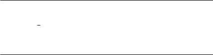
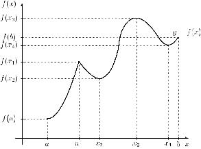
THEOREM 4.7 (intermediate-value theorem) Let function f : Df → R be continuous on the closed interval [a, b] Df . Moreover, let fmin be the smallest and fmax the largest value of function f for x [a, b]. Then for each y [fmin, fmax], there exists an x [a, b] such that f (x ) = y .
The geometrical meaning of Theorem 4.7 is illustrated in Figure 4.3. The graph of any line y = y [fmin, fmax] intersects at least once the graph of function f . For the particular value y chosen in Figure 4.3, there are two such values x1 and x2 with f (x1 ) = f (x2 ) = y .
Figure 4.3 Illustration of Theorem 4.7.
4.2 DIFFERENCE QUOTIENT AND THE DERIVATIVE
We now consider changes in the function value y = f (x) in relation to changes in the independent variable x. If we change the value x of the independent variable by some valuex, the function value may also change by some difference y, i.e. we have
y = f (x + x) − f (x).
We now consider the ratio of the changes y and x and give the following definition.
Definition 4.4 Let f : Df → R and x0, x0 + x (a, b) Df . The ratio
y |
= |
f (x0 + x) − f (x0) |
x |
x |
is called the difference quotient of function f with respect to points x0 + x and x0.

156 Differentiation
The quotient y/ x depends on the difference x and describes the average change of the value of function f between the points x0 and x0 + x. Let us now consider what happens when x → 0, i.e. the difference in the x values of the two points x0 + x and x0 becomes arbitrarily small.
Definition 4.5 Let f : Df → R. Then function f with y = f (x) is said to be differentiable at point x0 (a, b) Df if the limit
lim |
f (x0 + x) − f (x0) |
|
x |
||
x→0 |
exists. The above limit is denoted as
df (x0) = f (x0) dx
and is called the differential quotient or derivative of function f at point x0.
We only mention that one can define one-sided derivatives in an analogous manner, e.g. the left derivative of function f at some point x0 Df can be defined by considering only the left-side limit in Definition 4.5. If function f is differentiable at each point x of the open interval (a, b) Df , function f is said to be differentiable on the interval (a, b). Analogously, if function f is differentiable at each point x Df , function f is said to be differentiable.
If for any x Df the derivative f (x) exists, we obtain a function f with y = f (x) by assigning to each x Df the value f (x). We also say that function f is the first derivative of function f . If function f is continuous, we say that the original function f is continuously differentiable.
In economics, function f is also referred to as the marginal of f or the marginal function. It reflects the fact that the derivative characterizes the change in the function value provided that the change in the variable x is sufficiently small, i.e. it can be considered as ‘marginal’. This means that the marginal function can be interpreted as the approximate change in function f when variable x increases by one unit from x0 to x0 + 1, i.e.
f (x0) ≈ f (x0 + 1) − f (x0).
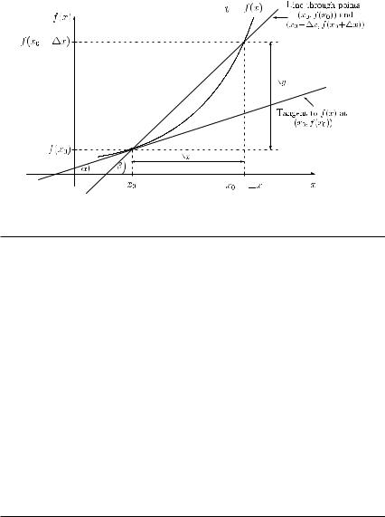
A geometric interpretation of the first derivative is as follows. The value f (x0) is the slope of the tangent to the curve y = f (x) at the point (x0, f (x0)) (see Figure 4.4). Consider the line through the points (x0, f (x0)) and (x0 + x, f (x0 + x)). For the slope of this line we have
y = tan β.
x
If x becomes smaller and tends to zero, the angle of the corresponding line and the x axis tends to α, and we finally obtain
f |
(x |
) |
= |
lim |
|
y |
= |
tan α. |
||
0 |
|
x |
||||||||
|
0 |
|
x |
→ |
|
|
||||
|
|
|
|
|
|
|
|
|
|
|
|
Differentiation |
157 |
Figure 4.4 |
Geometrical interpretation of the derivative f (x0). |
|
Example 4.7 Let function f : R → R with |
|
|
|
|
|
|
|
|
|
|
||||||||||||
|
|
|
|
|
2x |
for |
x < 1 |
|
|
|
|
|
|
|
|
|
|
|
|
|
||
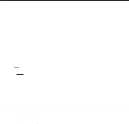
y = f (x) = 3 − x |
for |
1 ≤ x ≤ 2 |
|
|
|
|
|
|
|
|
|
|
||||||||||
be given and let x0 = 1. We obtain |
|
|
|
|
|
|
|
|
|
|
|
|
|
|
|
|||||||
lim |
|
|
f (x0 + x) − f (x0) |
|
lim |
|
2(x0 + x) − 2x0 |
|
lim |
|
2 x |
2 |
||||||||||
x |
→ |
− |
0 |
|
x |
|
= |
x |
→ |
− |
0 |
|
x |
|
= |
x |
→ |
− |
0 |
x |
= |
|
0 |
|
|
|
0 |
|
|
|
0 |
|
|||||||||||||
and |
|
|
|
|
|
|
|
|
|
|
|
|
|
|
|
|
|
|
|
|
|
|
lim |
|
|
f (x0 + x) − f (x0) |
= |
lim |
|
3 − (x0 + x) − (3 − x0) |
|
|
|
|
|
||||||||||
|
|
|
|
|
|
|
|
|||||||||||||||
x |
→ |
+ |
0 |
|
x |
|
x |
→ |
+ |
0 |
|
|
x |
|
|
|
|
|
|
|
|
|
0 |
|
|
|
0 |
|
|
= − |
|
|
|
|
|
|
|
|
|||||||
|
|
|
|
|
|
|
= x 0 |
|
0 x |
|
|
|
|
|
|
|
|
|
||||
|
|
|
|
|
|
|
|
lim |
|
− x |
|
1. |
|
|
|
|
|
|
|
|
||
|
|
|
|
|
|
|
|
|
|
|
|
|
|
|
|
|
|
|
||||
|
|
|
|
|
|
|
|
|
→ + |
|
|
|
|
|
|
|
|
|
|
|
|
|
Consequently, the differential quotient of function f at point x0 |
= 1 does not exist and |
|||||||||||||||||||||
function f |
is not differentiable at point x0 |
= 1. However, since both one-sided limits of |
||||||||||||||||||||
function f |
as x tends to 1 ± 0 exist and are equal to f (1) = 2, function f |
is continuous at |
||||||||||||||||||||
point x0 = 1.
The latter example shows that a function being continuous at point x0 is not necessarily differentiable at this point. However, the converse is true.
THEOREM 4.8 Let function f : Df → R be differentiable at point x0 Df . Then function f is continuous at x0.

158 Differentiation
4.3DERIVATIVES OF ELEMENTARY FUNCTIONS; DIFFERENTIATION RULES
Before giving derivatives of elementary functions, we consider an example for applying Definition 4.5.
Example 4.8 We consider function f : R → R with
f (x) = x3
and determine the derivative f at point x:
f (x) |
lim |
|
f (x + x) − f (x) |
= |
lim |
(x + x)3 − x3 |
||||||
|
|
|
|
|||||||||
= |
x |
→ |
0 |
x |
x |
→ |
0 |
|
|
x |
||
|
|
|
|
|||||||||
= |
lim |
|
x3 + 3x2 x + 3x( x)2 + ( x)3 − x3 |
|
||||||||
x |
→ |
0 |
x |
|
|
|
|
|
|
|
||
|
|
|
|
|
|
|
|
|||||
= |
lim |
|
x · [3x2 + 3x x + ( x)2] |
= |
3x2. |
|||||||
|
|
|||||||||||
x |
→ |
0 |
x |
|
|
|
|
|
|
|
||
|
|
|
|
|
|
|
|
|||||
The above formula for the derivative of function f with f (x) = x3 can be generalized to the case of a power function f with f (x) = xn, for which we obtain f (x) = nxn−1.
The determination of the derivative according to Definition 4.5 appears to be unpractical for frequent use in the case of more complicated functions. Therefore, we are interested in an overview on derivatives of elementary functions which we can use when investigating more complicated functions later. Table 4.1 contains the derivatives of some elementary functions of one variable.
Table 4.1 Derivatives of elementary functions
y = f (x) y = f (x) Df
C |
|
|
|
|
0 |
|
|
−∞ < x < ∞, |
C is constant |
||||||||||
xn |
nxn−1 |
−∞ < x < ∞, |
n N |
||||||||||||||||
xα |
αxα−1 |
0 < x < |
∞ |
, |
α |
|
R |
||||||||||||
|
x |
|
|
|
x |
|
x |
−∞ |
|
|
|
|
|
||||||
e |
x |
|
|
|
|
|
|
|
|
< x < |
∞ |
|
|
|
|||||
|
|
|
|
e |
|
|
|
|
|
|
|
|
|
|
|||||
a |
|
a ln a |
−∞ < x < ∞, a > 0 |
||||||||||||||||
ln x |
|
|
|
|
1 |
|
|
0 < x < ∞ |
|
|
|
||||||||
|
|
|
|
x |
|
|
|
|
|||||||||||
loga x |
|
|
|
|
1 |
|
|
0 < x < ∞, |
a > 0 |
||||||||||
|
|
|
|
|
|
||||||||||||||
|
x ln a |
||||||||||||||||||
sin x |
|
|
cos x |
−∞ < x < ∞ |
|
|
|
||||||||||||
cos x |
− sin x |
−∞ < x < ∞ |
|
|
|
||||||||||||||
|
|
|
|
|
|
1 |
|
|
x = |
π |
|
|
|
|
|
|
|||
tan x |
|
|
|
|
+ kπ , |
k Z |
|||||||||||||
|
cos2 x |
|
2 |
||||||||||||||||
cot x |
− |
|
|
1 |
|
|
x = kπ , |
|
|
k Z |
|||||||||
|
|
|
|||||||||||||||||
sin2 x |
|
|
|||||||||||||||||

Differentiation 159
Sum, product and quotient rules
Next, we present formulas for the derivative of the sum, difference, product and quotient of two functions.
THEOREM 4.9 Let functions f : Df → R and g : Dg → R be differentiable at x Df ∩Dg . Then the functions f + g, f − g, f · g and, for g(x) = 0, also function f /g are differentiable at point x, and we have:
(1)( f + g) (x) = f (x) + g (x);
(2)( f − g) (x) = f (x) − g (x);
(3)( f · g) (x) = f (x) · g(x) + f (x) · g (x);
(4)f (x) = f (x) · g(x) − f (x) · g (x) . g [g(x)]2
As a special case of part (3) we obtain: if f (x) = C, then (C · g) (x) = C · g (x), where C is a constant.
Example 4.9 Let function f : Df → R with
f (x) = 4x4 − 2x + ln x + √x
be given. Using √x = x1/2, we obtain
f (x) = 16x3 |
− 2 + |
1 |
+ |
|
1 |
|
|
|
|
√ |
|
. |
|||
x |
|
||||||
|
|
2 |
|
x |
|||
Example 4.10 In macroeconomics, it is assumed that for a closed economy
Y = C + I ,
where Y is the national income, C is the consumption and I is the investment. Assume that the consumption linearly depends on the national income, i.e. equation
C = a + bY
holds, where a and b are parameters. Here C (Y ) = b is called the marginal propensity to consume, a parameter which is typically assumed to be between zero and one. If we want to give the national income as a function depending on the investment, we obtain from
Y = a + bY + I
the function Y as
Y = Y (I ) = a + I . 1 − b

160 Differentiation
For the derivative Y (I ) we obtain
Y |
(I ) = |
dY |
= |
|
1 |
|
. |
dI |
1 |
− |
b |
||||
|
|
|
|
|
|
|
The latter result can be interpreted such that an increase in I by one unit leads to an increase of Y by 1/(1 − b) > 0 units.
Example 4.11 Let functions f : R → R and g : R → R with
f (x) = x2 |
|
and g(x) = ex |
|
|
|
|
||||||
be given. Then |
|
|
|
|
|
|
|
|
|
|||
( f · g) (x) = 2xex + x2ex = xex (x + 2) |
|
|
|
|
||||||||
|
f |
|
(x) |
|
2xex − x2ex |
|
|
xex (2 − x) |
|
|
x(2 − x) |
. |
g |
|
= |
(ex )2 |
= |
|
(ex )2 |
= |
|
ex |
|||
Derivative of composite and inverse functions
Next, we consider composite and inverse functions and give a rule to determine their derivatives.
THEOREM 4.10 Let functions f : Df |
→ R and g : Dg → R be continuous. Then: |
|||||||||||||||
(1) |
If function f is differentiable at point x Df and function g is differentiable at point |
|||||||||||||||
|
y = f (x) Dg , then function g ◦ f is also differentiable at point x and |
|||||||||||||||
|
|
|
(g ◦ f ) (x) = (g( f )) (x) = g ( f (x)) · f (x) |
(chain rule). |
||||||||||||
(2) |
Let function f be strictly monotone on Df and differentiable at point x Df with |
|||||||||||||||
|
f (x) |
= 0. Then the inverse function f −1 with x |
= f −1( y) is differentiable at point |
|||||||||||||
|
y = f (x) Df −1 and |
|
|
|
|
|
||||||||||
|
|
|
( f −1) ( y) |
1 |
1 |
|
. |
|
||||||||
|
|
|
|
|
|
|
|
|
||||||||
|
= f (x) |
= f f −1 |
( y) |
|
||||||||||||
|
|
|
|
|
|
|
|
|
|
|
|
|||||
An alternative formulation of the chain rule with h = g( y) and y = f (x) is given by |
||||||||||||||||
|
|
dh |
dh |
dy |
|
|
|
|
|
|
|
|||||
|
|
|
= |
|
|
|
· |
|
. |
|
|
|
|
|
||
|
|
dx |
|
dy |
dx |
|
|
|
|
|
||||||
The rule given in part (2) of Theorem 4.10 for the derivative of the inverse function f −1 can also be written as
(f −1) = |
|
1 |
|
|
. |
|
f |
|
f |
|
1 |
||
|
|
◦ |
|
− |
|
|

Differentiation 161
Example 4.12 Suppose that a firm produces only one product. The production cost, denoted by C, depends on the quantity x ≥ 0 of this product. Let
C = f (x) = 4 + ln(x + 1) + √3x + 1.
Then we obtain |
|
|
|
|
|
|
|
|
|
|
|
|
C = f (x) = |
df (x) |
= |
|
1 |
|
+ |
|
√ |
3 |
. |
||
|
|
|
|
|
|
|
||||||
dx |
x |
+ |
1 |
|||||||||
|
|
|||||||||||
|
|
|
|
|
|
|
2 |
3x + 1 |
||||
Assume that the firm produces x0 = 133 units of this product. We get
C |
(133) |
|
1 |
|
3 |
|
1 |
|
3 |
|
0.08246. |
|
= 134 |
+ |
2√ |
|
= 134 + |
40 ≈ |
|||||||
|
|
400 |
|
|||||||||
So, if the current production is increased by one unit, the production cost increases approximately by 0.08246 units.
Example 4.13 Let function g : Dg → R with
g(x) = cos [ln(3x + 1)]2
be given which is defined for x > −1/3, i.e. Dg = (−1/3, ∞). Setting
g = cos v, v = h2, h = ln y and y = (3x + 1),
application of the chain rule yields
g (x) = |
dg |
|
dv |
|
|
|
dh |
dy |
|
|
|
|||||
|
|
· |
|
|
· |
|
|
· |
|
, |
|
|
|
|
||
dv |
|
dh |
|
dy |
dx |
|
|
|
||||||||
and thus we get |
|
|
|
|
|
|
|
|
|
|
|
|
|
|||
g (x) = − sin [ln(3x + 1)]2 · 2 ln(3x + 1) · |
|
1 |
|
· 3 |
||||||||||||
|
|
|
||||||||||||||
3x |
+ |
1 |
||||||||||||||
|
|
|
|
6 |
|
|
|
|
|
|
|
|
|
|
||
= − |
|
|
|
|
· sin [ln(3x + 1)]2 · ln(3x + 1). |
|
||||||||||
|
|
|
|
|
|
|||||||||||
3x |
+ |
1 |
|
|
||||||||||||
|
|
|
|
|
|
|
|
|
|
|
|
|
|
|
||
|
|
|
|
|
|
|
|
|
|
|
|
|
|
|
|
|
By means of Theorem 4.10, we can also determine the derivatives of the inverse functions of the trigonometric functions. Consider the function f with
y = f (x) = sin x, x − |
π |
, |
π |
, |
|
|
|||
2 |
2 |
and the inverse function
x = f −1( y) = arcsin y.
162 Differentiation
Since f (x) = cos x, we obtain from Theorem 4.10, part (2):
(f |
−1) |
(y) |
|
1 |
|
|
|
1 |
. |
|
|
|
|
|
||||
= f (x) |
|
|
|
|
|
|
|
|
|
|||||||||
|
|
|
= cos x |
|
|
|
|
|||||||||||
|
|
|
|
|
|
|
|
|
|
|
|
|
|
|
|
|
||
|
|
|
|
|
|
|
|
|
|
|
|
|
|
|
|
|||
|
|
|
1 |
|
|
|
|
|
|
|
|
|
||||||
Because cos x = +√cos2 x = 1 − sin2 |
x = 1 − y2 for x (−π/2, π/2), we get |
|||||||||||||||||
(f |
−1) (y) |
|
|
|
|
|
|
|
, |
|
|
|
|
|
|
|
||
= |
|
|
|
|
|
|
|
|
|
|
|
|
||||||
|
|
|
1 − y2 |
|
|
|
|
|
|
|||||||||
and after interchanging variables x and y |
|
|
|
|
||||||||||||||
(f |
−1) |
(x) |
1 |
|
|
. |
|
|
|
|
|
|
||||||
|
|
|
|
|
|
|
|
|
|
|
|
|
||||||
= √ |
|
|
|
|
|
|
|
|
|
|
||||||||
|
|
|
1 − x2 |
|
|
|
|
|
||||||||||
Similarly, we can determine the derivatives of the inverse functions of the other trigonometric functions. We summarize the derivatives of the inverse functions of the trigonometric functions in the following overview:
|
= |
|
f |
|
= |
|
|
1 |
|
|
|
|
|
|
= { |
|
|
|
| − |
|
} |
|
|
f (x) |
arcsin x, |
|
√1 − x2 |
|
|
|
|
|
|||||||||||||||
|
(x) |
|
|
|
|
1 |
|
, |
|
Df |
|
x |
|
R |
|
1 < x < 1 |
|
; |
|||||
|
= |
|
f |
|
= − |
|
|
|
|
|
|
= { |
|
|
|
| − |
|
} |
|
||||
f (x) |
arccos x, |
|
√1 − x2 |
|
|
|
|
|
|||||||||||||||
|
(x) |
|
|
1 |
|
|
|
|
|
, |
Df |
|
x |
|
R |
|
1 < x < 1 |
|
; |
||||
f (x) = arctan x, |
f (x) = |
|
|
|
, |
|
|
|
Df |
= {x R | −∞ < x < ∞}; |
|||||||||||||
|
|
|
|
|
|||||||||||||||||||
1 |
+ |
x2 |
|||||||||||||||||||||
|
|
|
|
|
|
|
|
|
|
|
|
|
|
|
|
|
|
|
|
|
|
||
f (x) = arccot x, |
f (x) = − |
|
|
1 |
|
|
, |
Df |
= {x R | −∞ < x < ∞}. |
||||||||||||||
|
|
|
|
||||||||||||||||||||
1 |
+ |
x2 |
|||||||||||||||||||||
|
|
|
|
|
|
|
|
|
|
|
|
|
|
|
|
|
|
|
|
|
|
||
Logarithmic differentiation
As an application of the chain rule, we consider so-called logarithmic differentiation. Let
g(x) = ln f (x) |
with f (x) > 0. |
||
We obtain |
|
|
|
g (x) = [ln f (x)] = |
f (x) |
||
|
f (x) |
|
|
and thus |
|
|
|
f (x) = f (x) · g (x) = f (x) · [ln f (x)] .
Logarithmic differentiation is particularly useful when considering functions f of type f (x) = u(x)v(x),
i.e. both the basis and the exponent are functions depending on variable x.
Differentiation 163
Example 4.14 Let function f : Df → R with
f (x) = xsin x
be given. We set
g(x) = ln f (x) = ln xsin x = sin x · ln x.
Applying the formula of logarithmic differentiation, we get
g (x) = cos x · ln x + sin x · 1 x
and consequently
f (x) = f (x) · g (x) = xsin x |
1 |
|
|
cos x · ln x + sin x · |
|
. |
|
x |
|||
|
|
|
|
Higher-order derivatives
In the following we deal with higher-order derivatives. If function f with y = f (x) is again differentiable (see Definition 4.5), function
y = f (x) = df (x) = d2f (x) dx (dx)2
is called the second derivative of function f at point x. We can continue with this procedure and obtain in general:
y |
(n) |
= f |
(n) |
(x) = |
df n−1(x) |
= |
dnf (x) |
n ≥ 2, |
|||
|
|
|
|
|
, |
||||||
|
|
dx |
(dx)n |
||||||||
which denotes the nth derivative |
of function f |
at point x Df . Notice that we use |
|||||||||
f (x), f (x), f (x), and for n |
≥ 4, we use |
the |
notation f (n)(x). Higher-order deriva- |
||||||||
tives are used for instance in the next section when investigating specific properties of functions.
Example 4.15 Let function f : Df → R with
f (x) = 3x2 + 1 + e2x x

164 Differentiation
be given. We determine all derivatives until fourth order and obtain
f (x) = 6x − 1 + 2e2x x2
f (x) = 6 + 2 + 4e2x x3
f (x) = − 6 + 8e2x x4
f (4)(x) = 24 + 16e2x . x5
If the derivatives f (x0), f (x0), . . . , f (n)(x0) all exist, we say that function f is n times differentiable at point x0 Df . If f (n) is continuous at point x0, then function f is said to be n times continuously differentiable at x0. Similarly, if function f (n) is continuous, then function f is said to be n times continuously differentiable.
4.4 DIFFERENTIAL; RATE OF CHANGE AND ELASTICITY
In this section, we discuss several possibilities for characterizing the resulting change in the dependent variable y of a function when considering small changes in the independent variable x.
Definition 4.6 Let function f : Df → R be differentiable at point x0 (a, b) Df . The differential of function f at point x0 is defined as
dy = f (x0) · dx.
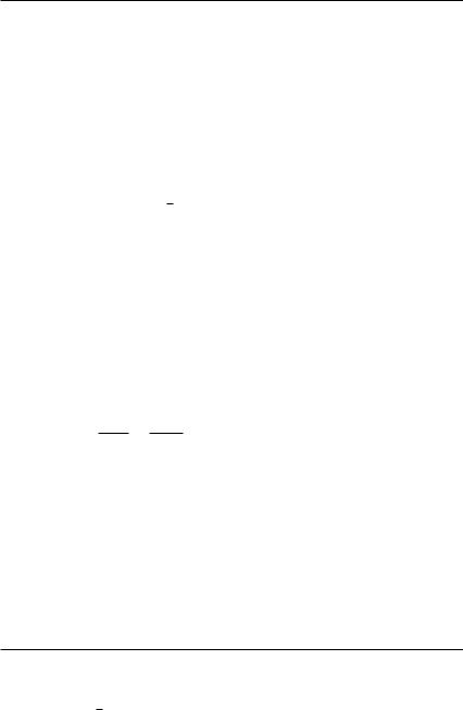
The differential is also denoted as df . Note that dy (or df ) is proportional to dx, with f (x0) as the factor of proportionality. The differential gives the approximate change in the function value at x0 when changing the argument by (a small value) dx (i.e. from x0 to x0 + dx), i.e.
y ≈ dy = f (x0) · dx.
The differential is illustrated in Figure 4.5.
The differential can be used for estimating the maximal absolute error in the function value when the independent variable is only known with some error. Let | x| = |dx| ≤ , then
| y| ≈ |dy| = |f (x0)| · |dx| ≤ |f (x0)| · .
Differentiation |
165 |
Figure 4.5 The differential dy.
Example 4.16 Let the length of an edge of a cube be determined as x = 7.5 ± 0.01 cm, i.e. the value x0 = 7.5 cm has been measured, and the absolute error is no greater than 0.01, i.e. |dx| = | x| ≤ = 0.01. For the surface of the cube we obtain
S0 = S(x0) = 6x02 = 337.5 cm2.
We use the differential to estimate the maximal absolute error of the surface and obtain
| S| ≈ |dS| ≤ |S (x0)| · = |12x0| · 0.01 = 0.9 cm2,
i.e. the maximal absolute error in the surface is estimated by 0.9 cm2, and we get
S0 ≈ 337.5 ± 0.9 cm3.
Moreover, for the estimation of the maximal relative error we obtain
|
S0 |
|
≈ |
|
S0 |
|
≤ |
|
S |
|
|
|
dS |
|
|
|
|
|
|
|
|
|
|
|
|
|
|
|
|
|
|
0.9
≈ 0.00267,
337.5
i.e. the maximal relative error is estimated by approximately 0.267 per cent.
We have already discussed that the derivative of a function characterizes the change in the function value for a ‘very small’ change in the variable x. However, in economics often a modified measure is used to describe the change of the value of a function f . The reason for this is that a change in the price of, e.g. bread by 1 EUR would be very big in comparison with the current price, whereas the change in the price of a car by 1 EUR would be very small. Therefore, economists prefer measures for characterizing the change of a function value in relation to this value itself. This leads to the introduction of the proportional rate of change of a function given in the following definition.

166 Differentiation
Definition 4.7 Let function f : Df → R be differentiable at point x0 (a, b) Df and f (x0) = 0. The term
ρf (x0) = f (x0) f (x0)
is called the proportional rate of change of function f : Df → R at point x0.
Proportional rates of change are often quoted in percentages or, when time is the independent variable, as percentages per year. This percentage rate of change is obtained by multiplying the value ρf (x0) by 100 per cent.
Example 4.17 Let function f : Df → R with
f (x) = x2e0.1x
be given. The first derivative of function f is given by
f (x) = 2xe0.1x + 0.1x2e0.1x = xe0.1x (2 + 0.1x)
and thus, the proportional rate of change at point x Df is calculated as follows:
ρ |
(x) |
f (x) |
|
xe0.1x (2 + 0.1x) |
2 |
|
0.1. |
|||||
|
|
|
|
|
|
|
|
|
||||
= f (x) |
= |
x2e0.1x |
= x |
+ |
||||||||
f |
|
|
||||||||||
We compare the proportional rates of change at points x0 = 20 and x1 = 2, 000. For x0 = 20, we get
ρf (20) = 2 + 0.1 = 0.2 20
which means that the percentage rate of change is 20 per cent. For x1 = 2, 000, we get
ρf (2, 000) = |
2 |
+ 0.1 = 0.101, |
2, 000 |
i.e. the percentage rate of change is 10.1 per cent. Thus, the second percentage rate of change is much smaller than the first one.
Definition 4.8 Let function f : Df → R be differentiable at point x0 (a, b) Df and f (x0) = 0. The term
εf (x0) = x0 · f (x0) = x0 · ρf (x0) f (x0)
is called the (point) elasticity of function f : Df → R at x0.

Differentiation 167
In many economic applications, function f represents a demand function and variable x
represents price or income. The (point) elasticity of function f |
corresponds to the ratio of the |
|||||||||
relative (i.e. percentage) changes of the function values of f and variable x: |
||||||||||
|
|
x0 |
f (x) |
|
|
f (x) x |
. |
|||
ε |
lim |
|
|
|
lim |
|
|
: |
|
|
|
x |
f (x0) |
x0 |
|||||||
f (x0) = |
x→0 f (x0) · |
= x→0 |
|
|
||||||
An economic function f is called elastic at point x0 Df if |εf (x0)| > 1. On the other hand, it is called inelastic at point x0 if |εf (x0)| < 1. In the case of |εf (x0)| = 1, function f is of unit elasticity at point x0.
In economics, revenue R is considered as a function of the selling price p by
R(p) = p · D( p),
where D is the demand function that is usually decreasing, i.e. if the price p rises, the quantity D sold falls. However, the revenue (as the product of price p and quantity D) may rise or fall. For the marginal revenue function, we obtain
R ( p) = p · D (p) + D( p).
Assume now that R ( p) > 0, i.e. from p · D ( p) + D( p) > 0 we get for D(p) > 0
εD( p) = p · D ( p) > −1,
D( p)
where due to D ( p) ≤ 0, we have |εD( p)| < 1. Thus, if revenue increases when the price increases, it must be at an inelastic interval of the demand function D = D( p), and in the inelastic case, a small increase in the price will always lead to an increase in revenue. Accordingly, in the elastic case, i.e. if |εD( p)| > 1, a small increase in price leads to a decrease in revenue. So an elastic demand function is one for which the quantity demanded is very responsive to price, which can be interpreted as follows. If the price increases by one per cent, the quantity demanded decreases by more than one per cent.
Example 4.18 We consider function f : (0, ∞) → R given by
f (x) = xx+1
and determine the elasticity of function f at point x Df . First, we calculate the first derivative f by applying logarithmic differentiation. We set
g(x) = ln f (x) = (x + 1) ln x. |
|
|
|
|
||||||||
Therefore, |
|
|
|
|
|
|
|
|
|
|
|
|
g (x) |
= [ |
ln f (x) |
|
= |
f (x) |
= |
ln x |
+ |
|
x + 1 |
. |
|
|
|
] |
f (x) |
|
|
|
x |
|
||||
Thus, we obtain for the first derivative
f (x) = f (x) · g (x) = xx+1 · ln x + x + 1 .
x
168 Differentiation
For the elasticity at point x Df , we obtain
|
|
|
x · f (x) |
x |
· |
xx+1 |
ln x |
+ |
x+1 |
|
|
|
|
|
|
|
ε |
(x) |
= |
= |
|
|
|
x |
= |
x ln x |
+ |
x |
+ |
1. |
|||
f |
|
f (x) |
|
|
|
xx+1 |
|
|
|
|
|
|||||
4.5 GRAPHING FUNCTIONS
To get a quantitative overview on a function f : Df → R resp. on its graph, we determine and investigate:
(1)domain Df (if not given)
(2)zeroes and discontinuities
(3)monotonicity of the function
(4)extreme points and values
(5)convexity and concavity of the function
(6)inflection points
(7)limits, i.e. how does the function behave when x tends to ±∞.
Having the detailed information listed above, we can draw the graph of function f . In the following, we discuss the above subproblems in detail.
In connection with functions of one variable, we have already discussed how to determine the domain Df and we have classified the different types of discontinuities. As far as the determination of zeroes is concerned, we have already considered special cases such as zeroes of a quadratic function. For more complicated functions, where finding the zeroes is difficult or analytically impossible, we give numerical procedures for the approximate determination of zeroes later in this chapter. We start with investigating the monotonicity of a function.
4.5.1 Monotonicity
By means of the first derivative f , we can determine intervals in which a function f is (strictly) increasing or decreasing. In particular, the following theorem can be formulated.
THEOREM 4.11 Let function f : Df → R be differentiable on the open interval (a, b) and let I = [a, b] Df . Then:
(1)Function f is increasing on I if and only if f (x) ≥ 0 for all x (a, b).
(2)Function f is decreasing on I if and only if f (x) ≤ 0 for all x (a, b).
(3)Function f is constant on I if and only if f (x) = 0 for all x (a, b).
(4)If f (x) > 0 for all x (a, b), then function f is strictly increasing on I .
(5)If f (x) < 0 for all x (a, b), then function f is strictly decreasing on I .
We recall from Chapter 3 that, if a function is (strictly) increasing or (strictly) decreasing on an interval I Df , we say that function f is (strictly) monotone on the interval I . Checking a

Differentiation 169
function f for monotonicity requires us to determine the intervals on which function f is monotone and strictly monotone, respectively.
Example 4.19 We investigate function f : R → R with
f (x) = ex (x2 + 2x + 1)
for monotonicity. Differentiating function f , we obtain
f (x) = ex (x2 + 2x + 1) + ex (2x + 2) = ex (x2 + 4x + 3).
To find the zeroes of function f , we have to solve the quadratic equation
x2 + 4x + 3 = 0
(notice that ex is positive for x R) and obtain
x1 = −2 + √4 − 3 = −1 and x2 = −2 − √4 − 3 = −3.
Since we have distinct zeroes (i.e. the sign of the first derivative changes ‘at’ each zero) and e.g. f (0) = 3 > 0, we get that f (x) > 0 for x (−∞, −3) (−1, ∞) and f (x) < 0 for
x (−3, −1). By Theorem 4.11 we get that function f is strictly increasing on the intervals (−∞, −3] and [−1, ∞) while function f is strictly decreasing on the interval [−3, −1].
4.5.2 Extreme points
First we give the definition of a local and of a global extreme point which can be either a minimum or a maximum.
Definition 4.9 A function f : Df → R has a local maximum (minimum) at point x0 Df if there is an interval (a, b) Df containing x0 such that
f (x) ≤ f (x0) ( f (x) ≥ f (x0), respectively) (4.1)
for all points x (a, b). Point x0 is called a local maximum (minimum) point. If inequality (4.1) holds for all points x Df , function f has at point x0 a global maximum
(minimum), and x0 is called a global maximum (minimum) point.
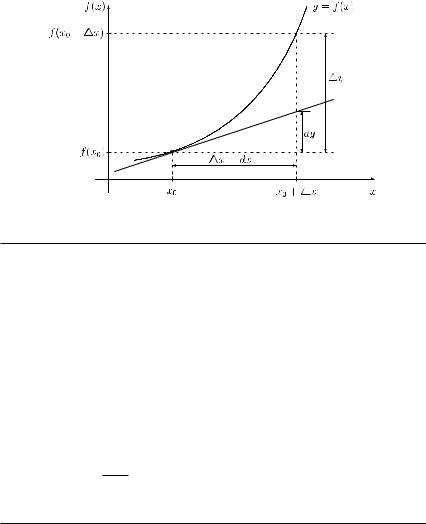
These notions are illustrated in Figure 4.6. Let Df = [a, b]. In the domain Df , there are two local minimum points x2 and x4 as well as two local maximum points x1 and x3. The global maximum point is x3 and the global minimum point is the left boundary point a. We now look for necessary and sufficient conditions for the existence of a local extreme point in the case of differentiable functions.
THEOREM 4.12 (necessary condition for local optimality) Let function f : Df → R be differentiable on the open interval (a, b) Df . If function f has a local maximum or local minimum at point x0 (a, b), then f (x0) = 0.
170 Differentiation
A point x0 (a, b) with f (x0) = 0 is called a stationary point (or critical point). In searching global maximum and minimum points for a function f in a closed interval I = [a, b] Df , we have to search among the following types of points:
(1)points in the open interval (a, b), where f (x) = 0 (stationary points);
(2)end points a and b of I ;
(3)points in (a, b), where f (x) does not exist.
Points in I according to (1) can be found by means of differential calculus. Points according to (2) and (3) have to be checked separately. Returning to Figure 4.6, there are three stationary points x2, x3 and x4. The local maximum point x1 cannot be found by differential calculus since the function drawn in Figure 4.6 is not differentiable at point x1.
Figure 4.6 Local and global optima of function f on Df = [a, b].
The following two theorems present sufficient conditions for so-called isolated local extreme points, for which in inequality (4.1) in Definition 4.9 the strict inequality holds for all x (a, b) different from x0. First, we give a criterion for deciding whether a stationary point is a local extreme point in the case of a differentiable function which uses only the first derivative of function f .
THEOREM 4.13 (first-derivative test for local extrema) |
Let function f : Df → R be |
differentiable on the open interval (a, b) Df and x0 |
(a, b) be a stationary point of |
function f . Then: |
|
(1)If f (x) > 0 for all x (a , x0) (a, b) and f (x) < 0 for all x (x0, b ) (a, b), then x0 is a local maximum point of function f .
(2)If f (x) < 0 for all x (a , x0) (a, b) and f (x) > 0 for all x (x0, b ) (a, b), then x0 is a local minimum point of function f .
(3)If f (x) > 0 for all x (a , x0) (a, b) and for all x (x0, b ) (a, b), then x0 is not a local extreme point of function f . The same conclusion holds if f (x) < 0 on both sides of x0.

Differentiation 171
For instance, part (1) of Theorem 4.13 means that, if there exists an interval (a , b ) around x0 such that function f is strictly increasing to the left of x0 and strictly decreasing to the right of x0 in this interval, then x0 is a local maximum point of function f . The above criterion requires the investigation of monotonicity properties of the marginal function of f . The following theorem presents an alternative by using higher-order derivatives to decide whether a stationary point is a local extreme point or not provided that the required higher-order derivatives exist.
THEOREM 4.14 (higher-order derivative test for local extrema) |
Let f : Df → R be n |
|
times continuously differentiable on the open interval (a, b) |
Df |
and x0 (a, b) be a |
stationary point. If |
|
|
f (x0) = f (x0) = f (x0) = · · · = f (n−1)(x0) = 0 and |
f (n)(x0) = 0, |
|
where number n is even, then point x0 is a local extreme point of function f , in particular:
(1)If f (n)(x0) < 0, then function f has at point x0 a local maximum.
(2)If f (n)(x0) > 0, then function f has at point x0 a local minimum.
Example 4.20 |
|
We determine all local extreme points of function f : (0, ∞) → R with |
|||||||||||
1 |
|
· ln2 3x. |
|
|
|
|
|
|
|
|
|||
f (x) = |
|
|
|
|
|
|
|
|
|
|
|||
x |
|
|
|
|
|
|
|
|
|||||
To check the necessary condition of Theorem 4.12, we determine |
|||||||||||||
|
|
|
1 |
|
1 |
1 |
|
1 |
|
||||
f (x) = − |
|
· ln2 |
3x + |
|
· 2 ln 3x · |
|
· 3 = |
|
|
· ln 3x(2 − ln 3x). |
|||
x2 |
x |
3x |
x2 |
||||||||||
From equality f (x) = 0, we obtain the following two cases which we need to consider.
Case a ln 3x = 0. Then we obtain 3x = e0 = 1 which yields x1 = 1/3.
Case b 2 − ln 3x = 0. Then we obtain ln 3x = 2 which yields x2 = e2/3.
To check the sufficient condition for x1 and x2 to be local extreme points according to Theorem 4.14, we determine f as follows:
f |
2 |
1 |
|
1 |
1 |
|
1 |
|
|||
(x) = − |
|
· ln 3x + |
|
· |
|
· 3 (2 − ln 3x) − |
|
· ln 3x · |
|
· 3 |
|
x3 |
x2 |
3x |
x2 |
3x |
|||||||
|
|
|
2 |
|
1 |
|
|
|
|
|
1 |
|
|
|
|
|
|
|||||
|
|
|
= − |
|
|
· ln 3x + |
|
|
(2 − ln 3x) − |
|
|
· ln 3x |
|
|
|
|||||||
|
|
|
x3 |
x3 |
x3 |
|
|
|
||||||||||||||
|
|
|
2 |
|
|
|
− 3 ln 3x + ln2 3x). |
|
|
|
|
|
|
|
|
|
|
|
||||
|
|
|
= |
|
· (1 |
|
|
|
|
|
|
|
|
|
|
|
||||||
|
|
|
x3 |
|
|
|
|
|
|
|
|
|
|
|
||||||||
In particular, we obtain |
|
|
|
|
|
|
|
|
|
|
|
|
||||||||||
|
|
1 |
|
|
|
|
|
|
|
|
|
|
1 |
|
|
54 |
|
54 |
||||
f |
|
|
= 54 > 0 and |
f |
|
|
e2 |
= |
|
· (1 |
− 3 · 2 + 22) = − |
|
< 0. |
|||||||||
3 |
3 |
e6 |
e6 |
|||||||||||||||||||
Hence, x1 = 1/3 is a local minimum point with f (x1) = 0, and x2 = e2/3 is a local maximum point with f (x2) = 12/e2.
172 Differentiation
Example 4.21 A monopolist (i.e. an industry with a single firm) producing a certain product has the demand–price function (also denoted as the inverse demand function)
p(x) = −0.04x + 200,
which describes the relationship between the (produced and sold) quantity x of the product and the price p at which the product sells. This strictly decreasing function is defined for 0 ≤ x ≤ 5, 000 and can be interpreted as follows. If the price tends to 200 units, the number of customers willing to buy the product tends to zero, but if the price tends to zero, the sold quantity of the product tends to 5,000 units. The revenue R of the firm in dependence on the output x is given by
R(x) = p(x) · x = (−0.04x + 200) · x = −0.04x2 + 200x.
Moreover, let the cost function C describing the cost of the firm in dependence on the produced quantity x be given by
C(x) = 80x + 22, 400.
This yields the profit function P with
P(x) = R(x) − C(x) = −0.04x2 + 200x − (80x + 22, 400) = −0.04x2 + 120x − 22, 400.
We determine the production output that maximizes the profit. Looking for stationary points we obtain
P (x) = −0.08x + 120 = 0
which yields the point
xP = 1, 500.
Due to
P (xP ) = −0.08 < 0,
the output xP = 1, 500 maximizes the profit with P(1, 500) = 67, 600 units. Points with P(x) = 0 (i.e. revenue R(x) is equal to cost C(x)) are called break-even points. In the example, we obtain from P(x) = 0 the equation
x2 − 3, 000x + 560, 000 = 0,
which yields the roots (break-even points)
x1 = 1, 500 − 1, 690, 000 = 200 and x2 = 1, 500 + 1, 690, 000 = 2, 800,
i.e. an output x (200; 2, 800) leads to a profit for the firm. Finally, we mention that when maximizing revenue, one gets from
R (x) = −0.08x + 200 = 0

Differentiation 173
the stationary point
xR = 2, 500,
which is, because R (2, 500) = −0.08 < 0, indeed the output that maximizes revenue. However, in the latter case, the profit is only P(2, 500) = 27, 600 units.
Example 4.22 The cost function C : R+ → R of an enterprise producing a quantity x of a product is given by
C(x) = 0.1x2 − 30x + 25, 000.
Then, the average cost function Ca measuring the cost per unit produced is given by
Ca(x) = |
C(x) |
= 0.1x − 30 + |
25, 000 |
. |
|
x |
|
x |
|||
We determine local minimum points of the average cost function Ca. We obtain
a |
|
= |
|
− |
25, 000 |
|
|
|
x2 |
|
|||
C |
(x) |
|
0.1 |
|
|
. |
The necessary condition for a local extreme point is Ca(x) = 0. This corresponds to
0.1x2 = 25, 000
which has the two solutions
x1 = 500 and x2 = −500.
Since x2 DC , the only stationary point is x1 = 500. Checking the sufficient condition, we obtain
C |
|
(x) |
= |
2 |
· |
|
25, 000 |
|
|
|
x3 |
||||||||
|
a |
|
|
|
|||||
and |
|
|
|
|
|
|
|
|
|
C |
(500) |
= |
50, 000 |
> 0, |
|||||
|
|||||||||
|
|||||||||
|
a |
|
|
125, 000, 000 |
|||||
i.e. the produced quantity x1 = 500 minimizes average cost with Ca(500) = 70.
Example 4.23 A firm wins an order to design and produce a cylindrical container for transporting a liquid commodity. This cylindrical container should have a given volume V0. The cost of producing such a cylinder is proportional to its surface. Let R denote the radius and H denote the height of a cylinder. Among all cylinders with given volume V0, we want
174 Differentiation
to determine that with the smallest surface S (i.e. that with lowest cost). We know that the volume is obtained as
V0 = V (R, H ) = π R2H , |
(4.2) |
||
and the surface can be determined by the formula |
|
||
S = S(R, H ) = 2π R2 + 2π RH . |
(4.3) |
||
From formula (4.2), we can eliminate variable H which yields |
|
||
H = |
V0 |
|
|
|
. |
(4.4) |
|
π R2 |
|||
Substituting the latter term into formula (4.3), we obtain the surface as a function of one variable, namely in dependence on the radius R, since V0 is a constant:
|
V0 |
|
|
|
S = S(R) = 2π R2 + 2π R · |
π R2 |
= 2 π R2 + |
R |
. |
Now we look for the minimal value of S(R) for 0 < R < ∞. For applying Theorems 4.12 and 4.14, we determine the first and second derivatives of function S = S(R):
|
V0 |
|
|
|
|
2V0 |
. |
|
S (R) = 2 |
2π R − |
|
and |
S (R) = 2 |
2π + |
|
||
R2 |
R3 |
|||||||
Setting S (R) = 0 yields |
|
|
|
|
|
|
||
2π R3 − V0 = 0 |
|
|
|
|
|
(4.5) |
||
and thus the stationary point is obtained as follows:
R1 = 3 V0 . 2π
Notice that the other two roots of equation (4.5) are complex and therefore not a candidate point for a minimal surface of the cylinder. Moreover, we obtain
S (R1) = 2(2π + 4π ) = 12π > 0,
i.e. the surface becomes minimal for the radius R1. One can also argue without checking the sufficient condition that the only stationary point with a positive radius must be a minimum point since, both as R → 0 and as R → ∞, the surface of the cylinder tends to infinity so that for R1, the surface must be at its minimal value. Determining the corresponding value for the height, we obtain from equality (4.4)
|
= |
π R12 = |
3 |
V0 |
|
2 = |
|
π V |
2/3 |
= |
|
· |
|
|
|
= |
|
· |
|
|
|
= |
|
|||||
|
|
|
|
π |
|
2π |
|
|||||||||||||||||||||
H1 |
|
|
V0 |
V0 |
|
|
|
V0 |
· (2π )2/3 |
|
22/3 |
|
3 V0 |
2 |
|
3 V0 |
|
2R1. |
||||||||||
|
|
|
|
|
|
|
|
|
|
|
|
|
|
|
|
|
|
|
|
|
|
|
||||||
|
|
|
|
π |
|
|
|
|
|
· |
0 |
|
|
|
|
|
|
|
|
|
|
|
|
|
|
|||
|
|
|
|
2π |
|
|
|
|
|
|
|
|
|
|
|
|
|
|
|
|
|
|
||||||
Thus, the surface of a cylinder with given volume is minimal if the height of the cylinder is equal to its diameter, i.e. H = 2R.
Differentiation 175
4.5.3 Convexity and concavity
The definition of a convex and a concave function has already been given in Chapter 3. Now, by means of differential calculus, we can give a criterion to check whether a function is (strictly) convex or concave on a certain interval I .
THEOREM 4.15 |
Let function f : Df → R be twice differentiable on the open interval |
|||
(a, b) Df and let I = [a, b]. Then: |
|
|
||
(1) |
Function f |
is convex on I if and only if f (x) ≥ 0 |
for all |
x (a, b). |
(2) |
Function f |
is concave on I if and only if f (x) ≤ 0 |
for all |
x (a, b). |
(3)If f (x) > 0 for all x (a, b), then function f is strictly convex on I .
(4)If f (x) < 0 for all x (a, b), then function f is strictly concave on I .
Example 4.24 Let function f |
: R → R with |
|
f (x) = aebx , |
a, b R+ \ {0} |
|
be given. We obtain |
|
|
f (x) = abebx |
and |
f (x) = ab2ebx . |
For a, b > 0, we get f (x) > 0 and f (x) > 0 for all x Df , i.e. function f is strictly increasing and strictly convex. In this case, we say that function f has a progressive growth (since it grows faster than a linear function, which has a proportionate growth).
Consider now function g : R+ → R with
g(x) = a ln(1 + bx), |
|
a, b R+ \ {0}. |
|
|
|
|||||
We obtain |
|
|
|
|
|
|
|
|
|
|
g (x) = |
|
ab |
|
g (x) = − |
|
ab2 |
||||
|
|
|
|
and |
|
|
|
. |
||
1 |
+ |
bx |
(1 |
+ |
bx)2 |
|||||
|
|
|
|
|
|
|
|
|
||
For a, b > 0, we get g (x) > 0 and g (x) < 0 for all x Dg , i.e. function g is strictly increasing and strictly concave. In this case, we say that function g has degressive growth.
Example 4.25 We investigate function f : R → R with
2x
f (x) =
x2 + 1

176 |
Differentiation |
|
|
|
|
|
|
|
|
|
|
|
|
||||||||
for convexity and concavity. We obtain |
|
|
|
|
|
|
|
|
|
||||||||||||
f |
(x) |
= |
|
2(x2 + 1) − 2x · 2x |
= |
2 |
· |
|
1 − x2 |
|
|
|
|
|
|||||||
|
|
|
(x2 + 1)2 |
|
|
|
|
||||||||||||||
|
|
|
|
|
(x2 + 1)2 |
|
|
|
|
|
|
||||||||||
f |
(x) |
= |
2 |
· |
−2x(x2 + 1)2 − (1 − x2) · 2 · (x2 + 1) · 2x |
||||||||||||||||
|
|
|
|||||||||||||||||||
|
|
|
|
|
|
|
|
(x2 + 1)4 |
|
− |
|
· |
|
||||||||
|
|
|
2 |
|
(x |
|
+ 1) · − 2x(x2 |
+ 1 4− |
|
x2) |
|||||||||||
|
|
= |
|
|
· |
|
2 |
|
|
2 |
|
|
) |
(1 |
|
|
|
4x |
|||
|
|
|
|
|
|
|
|
(x |
+ |
1) |
|
|
|
|
|
|
|
||||
|
|
|
|
|
|
x3 |
− 3x |
|
|
|
|
|
|
|
|
|
|
|
|||
|
|
= |
4 |
· |
. |
|
|
|
|
|
|
|
|
|
|
|
|
||||
|
|
(x2 |
+ 1)3 |
|
|
|
|
|
|
|
|
|
|
|
|
||||||
|
|
|
|
|
|
|
|
|
|
|
|
|
|
|
|
|
|||||
To find the zeroes of the second derivative f , we have to solve the cubic equation
x3 − 3x = x · (x2 − 3) = 0
which yields the solutions
x1 = 0, x2 = √3 and x3 = −√3.
√
Since e.g. f (1) = 4 · (1 − 3)/23 = −1 < 0, we have f (x) < 0 for x (x , x ) = (0, 3),
√ 1 2
i.e. by Theorem 4.15, function f is strictly concave on the interval [0, 3]. Moreover, since we have distinct zeroes, the sign of the second derivative changes√ ‘at’√each zero, and by Theorem 4.15 we obtain:√ function√ f is strictly convex on [− 3, 0] [ 3, ∞) and strictly concave on (−∞, − 3] [0, 3].
To decide whether a function is convex or concave, the following notion of an inflection point can be helpful.
Definition 4.10 Let function f : Df → R be twice differentiable on the open interval (a, b) Df . Point x0 (a, b) is called an inflection point of function f when f changes at x0 from being convex to being concave or vice versa, i.e. if there is an interval (a , b ) (a, b) containing x0 such that either of the following two conditions
holds:
(1) |
f (x) ≥ 0 |
if a |
< x < x0 |
and |
f (x) ≤ 0 |
if x0 |
< x < b |
or |
(2) |
f (x) ≤ 0 |
if a |
< x < x0 |
and |
f (x) ≥ 0 |
if x0 |
< x < b . |
|
Consequently, if the second derivative changes the sign ‘at’ point x0, then point x0 is an inflection point of function f . The notion of an inflection point is illustrated in Figure 4.7. Next, we give a criterion for an inflection point of function f .
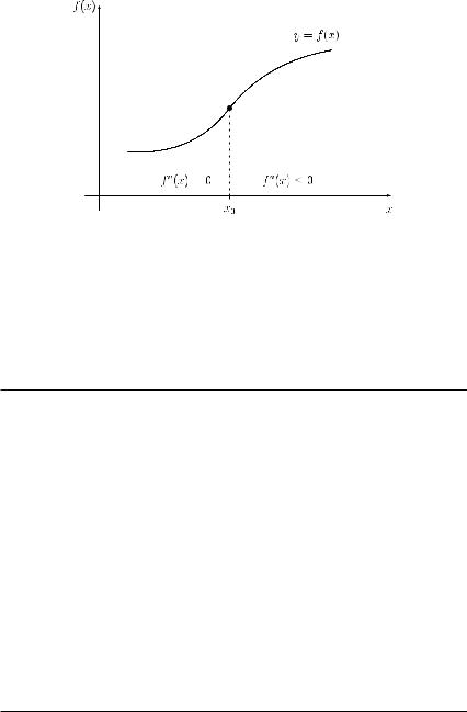
Differentiation 177
Figure 4.7 Inflection point x0 of function f .
THEOREM 4.16 Let function f : Df → R be n times continuously differentiable on the open interval (a, b) Df . Point x0 (a, b) is an inflection point of function f if and only if
f (x0) = f (x0) = · · · = f (n−1)(x0) = 0 |
and |
f (n)(x0) = 0, |
where n is odd. |
|
|
Example 4.26 We consider function f : R → R with
f (x) = x4 + 2x3 − 12x2 + 4 = 0
and determine inflection points. We obtain
f (x) = 4x3 + 6x2 − 24x and f (x) = 12x2 + 12x − 24.
In order to solve f (x) = 0, we have to find the roots of the quadratic equation
x2 + x − 2 = 0,
which gives x1 = 1 and x2 = −2 as candidates for an inflection point. Using
f (x) = 24x + 12,
we obtain f (1) = 36 = 0 and f (−2) = −36 = 0, i.e. both points x1 = 1 and x2 = −1 are inflection points of function f .

178 Differentiation
4.5.4 Limits
We have already discussed some rules for computing limits of sums, differences, products or quotients of functions. However, it was necessary that each of the limits exists, i.e. each of the limits was a finite number. The question we consider now is what happens when we want to determine the limit of a quotient of two functions, and both limits of the function in the numerator and the function in the denominator tend to ∞ as x tends to a specific value x0. The same question arises when both functions in the numerator and in the denominator tend to zero as x approaches some value x0.
Definition 4.11 If in a quotient both the numerator and the denominator tend to zero as x tends to x0, we call such a limit an indeterminate form of type “0/0”, and we write
lim f (x) = “ 0/0”.
x→x0 g(x)
The notion ‘indeterminate form’ indicates that the limit cannot be found without further examination. There exist six further indeterminate forms as follows:
“∞/∞”, “0 · ∞”, “∞ − ∞”, “00”, “∞0”, “1∞”.
For the two indeterminate forms “0/0” and “∞/∞”, the limit can be found by means of the following rule.
THEOREM 4.17 (Bernoulli–l’Hospital’s rule) Let functions f : Df → R and g : Dg → R both tend to zero as x tends to x0, or f and g both tend to ∞ as x tends to x0. Moreover, let f and g be continuously differentiable on the open interval (a, b) Df ∩ Dg containing x0 and g (x) = 0 for x (a, b). Then
lim |
f (x) |
lim |
f (x) |
= L. |
x→x0 g(x) |
= x→x0 g (x) |
|||
Here either the limit exists (i.e. value L is finite) or the limit does not exist.
It may happen that after application of Theorem 4.17, we still have an indeterminate form of type “0/0” or “∞/∞”. In that case, we apply Theorem 4.17 repeatedly as long as we have found L. Moreover, we mention that Theorem 4.17 can be applied under appropriate assumptions also to one-sided limits (i.e. x → x0 + 0 or x → x0 − 0) as well as to the cases x → −∞ and x → ∞. To illustrate Theorem 4.17, consider the following example.
Example 4.27 We determine the limit
L lim |
esin 2x − e2x |
, |
||||
|
||||||
= x |
→ |
0 |
sin 2x |
− |
2x |
|
|
|
|
||||


180 |
Differentiation |
|
|
|
|
||
|
|
|
|||||
Example 4.28 |
We determine |
||||||
|
= x→∞ |
|
|
|
|
− |
|
|
|
− |
|
||||
L |
lim |
3 x3 |
|
2x2 |
|
x . |
|
Obviously, this is an indeterminate form of type “∞ − ∞”. We reduce this form to the type “0/0” without the above general transformation. Instead of it, we perform for x = 0 the following algebraic manipulation:
3 |
x3 |
− 2x2 − x = 'x3 1 − x ( |
− x = x 1 − x |
− x |
“∞ − ∞” |
|||||||||||||||||||||||||||||
|
|
|
|
|
|
|
|
|
|
|
|
2 |
|
|
|
1/3 |
|
|
|
|
2 |
1/3 |
|
|
|
|
||||||||
|
|
|
|
|
|
|
= x % 1 − x |
|
|
|
− 1& . |
|
|
|
|
|
|
|
|
“ ∞ · 0” |
||||||||||||||
|
|
|
|
|
|
|
|
|
|
|
|
|
|
2 |
|
|
1/3 |
|
|
|
|
|
|
|
|
|
|
|
|
|
||||
Thus we obtain |
|
|
|
|
|
|
|
|
|
|
|
|
|
|
|
|
|
|
|
|
|
|
|
|
|
|
|
|
||||||
x |
|
|
|
|
|
|
|
|
|
|
|
|
x |
|
|
|
|
|
|
1/3 − 1 |
|
|
|
|
|
|
|
|
||||||
lim |
3 |
x3 |
− |
2x2 |
− |
x |
lim |
|
|
1 − 2x |
|
|
|
|
|
|
|
|
|
|||||||||||||||
|
→∞ |
|
= |
|
→∞ |
|
|
x |
|
|
|
|
|
|
|
|
|
|
|
|
||||||||||||||
|
|
|
|
|
|
|
|
|
|
|
|
|
|
|
|
|
|
|
|
|
|
1 |
|
|
|
|
|
|
|
|
|
|
|
|
which is an indeterminate form of type “0/0”. By applying Theorem 4.17, we obtain |
||||||||||||||||||||||||||||||||||
|
|
= →∞ |
|
|
− x2 |
|
|
|
|
|
= →∞ %− 3 |
− x |
|
& = − 3 |
|
|||||||||||||||||||
|
|
|
1 |
|
|
2 |
|
|
−2/3 |
|
2 |
|
|
|
|
|
|
|
|
|
|
|
|
|
|
|
|
|
|
|
||||
L |
|
xlim |
3 |
1 − x |
|
|
· |
x2 |
|
|
|
|
xlim |
|
|
2 |
1 |
2 |
|
−2/3 |
|
2 |
. |
|
||||||||||
|
|
|
|
1 |
|
|
|
|
|
|
|
|
|
|
|
|
|
|
|
|
|
|||||||||||||
If we have an indeterminate form of type “00”, “∞0” or “1∞”, i.e. the limit to be determined has the structure
L = lim g(x)f (x)
x→x0
with g(x) > 0, we take the natural logarithm on both sides of the equation
y(x) = g(x)f (x)
and obtain
ln y(x) = ln g(x)f (x) = f (x) · ln g(x).
If now x tends to x0, we obtain an indeterminate form of type “0 · ∞” which we can already treat. Suppose that this limit exists and let
L1 = lim f (x) · ln g(x) ,
x→x0
then we finally get
L = eL1 .
182 Differentiation
Figure 4.8 Graph of function f with f (x) = (x2 + 5x + 22)/(x − 2).
From f (x) = x2 + 5x + 22 = 0, we obtain the roots
x1 = − |
5 |
+ |
25 |
− 22 and x2 = − |
5 |
− |
25 |
− 22. |
||||
2 |
4 |
|
2 |
4 |
||||||||
Since |
|
|
|
|
|
|
|
|
|
|
||
|
25 |
− 22 = − |
63 |
|
< 0, |
|
|
|
|
|||
|
|
|
|
|
|
|
||||||
44
there do not exist real zeroes of function f . We obtain for the first and second derivatives
f (x) |
= |
(2x + 5)(x − 2) − (x2 + 5x + 22) |
= |
|
x2 − 4x − 32 |
|
|
|
||||||||||
|
|
(x |
− |
2)2 |
|
|
(x |
− |
2)2 |
|
|
|
|
|||||
|
|
|
|
|
|
|
|
|
|
|
||||||||
and |
|
|
|
|
|
|
|
|
|
|
|
|
|
|
|
|
|
|
f (x) |
|
|
(2x − 4)(x − 2)2 − 2(x − 2)(x2 − 4x − 32) |
|
|
|
72 |
. |
||||||||||
= |
|
|
= (x |
|
||||||||||||||
|
|
|
|
(x |
− |
2)4 |
|
|
|
|
|
− |
2)3 |
|
||||
|
|
|
|
|
|
|
|
|
|
|
|
|
||||||
Setting f (x) = 0, we obtain x2 − 4x − 32 = 0 which yields the stationary points x3 = 2 + √4 + 32 = 8 and x4 = 2 − √4 + 32 = −4.

Differentiation 183
From f (x3) > 0, we get that x3 = 8 is a local minimum point with f (x3) = 21, and from f (x4) < 0, we get that x4 = −4 is a local maximum point with f (x4) = −3. Since f (x) > 0
for all x (−∞, −4) (8, ∞), function f |
is strictly increasing on (−∞, −4] [8, ∞). |
For x (−4, 2) (2, 8), we have f (x) < |
0, and thus function f is strictly decreasing |
on [−4, 2) (2, 8]. To determine candidates for an inflection point, we set f (x) = 0. The latter equation has no solution, and thus function f does not have an inflection point. Because f (x) > 0 for x (2, ∞), function f is strictly convex on the interval (2, ∞). Since f (x) < 0 for x (−∞, 2), function f is strictly concave on the interval (−∞, 2). Moreover,
xlim |
f (x) = ∞ and |
x |
lim f (x) = −∞. |
→∞ |
|
|
→−∞ |
The graph of function f is given in Figure 4.8.
Example 4.31 Let the relationship between the price p of a good and the resulting demand D for this good be given by the demand function D = D(p), where
D |
= |
400 |
− |
10p |
, |
0 |
≤ |
p |
≤ |
40. |
(4.6) |
|
|
p |
+ |
5 |
|||||||||
|
|
|
|
|
|
|
||||||
|
|
|
|
|
|
|
|
|
|
|
|
|
First, we determine the extreme points of function D = D( p) and check the function for monotonicity as well as concavity or convexity. We obtain
D ( p) |
|
−10( p + 5) − (400 − 10p) · 1 |
|
|
450 |
. |
|||
= |
|
= − ( p |
|
||||||
|
(p |
+ |
5)2 |
+ |
5)2 |
|
|||
|
|
|
|
||||||
Thus D ( p) = 0 for all p [0, 40], and therefore function D = D( p) cannot have an extreme point since the necessary condition for its existence is not satisfied. Moreover, since D ( p) < 0 for all p (0, 40), function D = D( p) is strictly decreasing on the closed interval [0, 40]. Checking function D = D( p) for convexity and concavity, respectively, we obtain
D ( p) = −450( p + 5)−3 · (−2) = |
|
900 |
> 0 |
|
( p |
+ |
5)3 |
||
|
|
|
|
|
for all p (0, 40). Therefore, function D = D( p) is strictly convex on the closed interval [0, 40].
Next, we check function D = D( p) for elasticity. We obtain
ε |
|
( p) |
= |
|
p · D ( p) |
|
|
450p( p + 5) |
|
|
|
|
45p |
|
|
. |
||||
D |
D( p) |
= − ( p |
|
= − (p |
|
5)(40 |
|
|
||||||||||||
|
|
|
+ |
5)2 |
(400 |
− |
10p) |
+ |
− |
p) |
||||||||||
|
|
|
|
|
|
|
|
|
|
|
|
|
|
|
|
|
||||
We can determine points where function D = D( p) changes between being elastic and inelastic, i.e. we can check, where equality |εD( p)| = 1 holds and obtain
45p
= 1.
( p + 5)(40 − p)
Thus,
( p + 5)(40 − p) = 45p
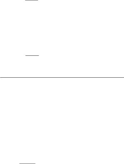
184 Differentiation
which yields the quadratic equation
p2 + 10p − 200 = 0
with the two solutions
p1 = −5 + √25 + 200 = −5 + 15 = 10 and p2 = −5 − 15 = −20 < 0.
Solution p2 does not belong to the domain DD of function D = D( p). Hence, for p = 10, function D is of unit elasticity. Since |εD(p)| < 1 for p [0, 10) and |εD( p)| > 1 for p (10, 40], we get that function D = D( p) is inelastic for p [0, 10) and elastic for p (10, 40].
Finally, we look for the function p = p(D) giving the price in dependence on the demand D. Since function D(p) is strictly decreasing on the closed interval [0, 40], the inverse demand function p = p(D) exists. Solving equation (4.6) for p, we obtain
D(p + 5) = 400 − 10p p(D + 10) = 400 − 5D
p = 400 − 5D . D + 10
Since D = D( p) is strictly monotone, the inverse function p = p(D) is strictly monotone as well. Because D(0) = 80 and D(40) = 0 (see also the inequality in (4.6)), function p = p(D) is defined for D [0, 80].
4.6 MEAN-VALUE THEOREM
Before presenting the mean-value theorem of differential calculus, we start with a special case.
THEOREM 4.18 (Rolle’s theorem) Let function f : Df → R be continuous on the closed interval [a, b] Df with f (a) = f (b) = 0 and differentiable on the open interval (a, b). Then there exists a point x (a, b) with f (x ) = 0.
Geometrically, Rolle’s theorem says that in the case of f (a) = f (b), there exists an interior point x of the interval (a, b), where the tangent line is parallel to the x axis. In other words, there is at least one stationary point in the open interval (a, b). The mean-value theorem of differential calculus generalizes Rolle’s theorem to the case f (a) = f (b).
THEOREM 4.19 (mean-value theorem of differential calculus) Let function f : Df → R be continuous on the closed interval [a, b] Df and differentiable on the open interval (a, b). Then there exists at least one point x (a, b) such that
f (x ) = f (b) − f (a) . b − a
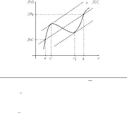
Differentiation 185
The mean-value theorem of differential calculus is illustrated in Figure 4.9. In this case, we have two points x1 (a, b) and x2 (a, b) with the property that the derivative of function f at each of these points is equal to the quotient of f (b) − f (a) and b − a.
The mean-value theorem of differential calculus can be used e.g. for the approximate calculation of function values.
Figure 4.9 Mean-value theorem of differential calculus.
√
Example 4.32 Using the mean-value theorem, we compute 3 29. Let us consider function f : R+ → R with
√
f (x) = 3 x.
We get
f (x) = 1 · x−2/3. 3
Applying the mean-value theorem with a = 27 and b = 29, we get
f (b) − f (a) |
3 |
|
|
3 |
|
|
3 |
|
|
− 3 |
|
|
|
|
|||
|
√29 |
− √27 |
|
√29 |
|
f (x ) |
1 |
(x )−2/3 |
|||||||||
b |
− |
a |
= 29 |
− |
27 |
= |
2 |
|
= |
= 3 · |
|||||||
|
|
|
|||||||||||||||
which can be rewritten as
3 |
|
|
1 |
|
|
|
|
||
√29 |
= 3 + |
|
· (x )−2/3 · 2. |
|
3 |
||||
Using x = 27 (notice that x is not from the open interval (27, 29), but it can be chosen since function f is differentiable at x = a = 27 and moreover, the value of function f is

186 Differentiation |
|
|
|
|
|
|
|
|
||
easily computable at this point), we get |
|
|
|
|
|
|||||
√ |
|
1 |
1 |
|
1 |
|
2 |
|
2 |
|
3 |
29 ≈ 3 + |
· 2 = 3 + |
· |
= 3 + |
≈ 3.074. |
|||||
|
3 · |
272/3 |
3 |
(33)2/3 |
27 |
|||||
Example 4.33 A vehicle starts at time zero and s(t) gives the distance from the starting point (in metres) in dependence on time t (in seconds). It is known that s(t) = t2/2 and let a = 0 and b = 20. Then the mean-value theorem reads as
s(20) |
− |
s(0) |
= |
21 · 202 − 0 |
= |
200 |
= 10 = s (t ) = t . |
||
20 |
− |
0 |
|
20 |
|
20 |
|||
|
|
|
|
|
|
|
|
|
|
The left-hand side fraction gives the average velocity of the vehicle in the interval [0, 20] which is equal to 10 m per second. The mean-value theorem implies that there is at least one value t (0, 20), where the current velocity of the vehicle is equal to 10 m/s. In the above example, it happens at time t = 10.
4.7 TAYLOR POLYNOMIALS
Often it is necessary to approximate as closely as possible a ‘complicated’ function f by a polynomial Pn of some degree n. One way to do this is to require that all n derivatives of function f and of the polynomial Pn, as well as the function values of f and Pn, coincide at some point x = x0 provided that function f is sufficiently often differentiable.
Before considering the general case, we discuss this question for some small values of n. First consider n = 1. In this case, we approximate function f around x0 by a linear function (straight line)
P1(x) = f (x0) + f (x0) · (x − x0).
Obviously, we have P1(x0) = f (x0) and P1(x0) = f (x0). For n = 2, we approximate function f by a quadratic function (parabola) P2 with
P2(x) = f (x0) + f (x0) · (x − x0) + f (x0) · (x − x0)2. 2!
In this case, we also have P2(x0) = f (x0), P2(x0) = f (x0) and additionally P2 (x0) = f (x0). Suppose now that function f is sufficiently often differentiable, and we wish to approximate function f by a polynomial Pn of degree n with the requirements listed above.
THEOREM 4.20 |
Let function f : Df → R be n + 1 times differentiable on the open interval |
|||||||||||||
(a, b) Df containing points x0 and x. Then function f can be written as |
||||||||||||||
f (x) = f (x0) + |
f |
(x0) |
· (x − x0) + |
f |
(x0) |
· (x − x0) |
2 |
+ · · · |
||||||
|
|
1 |
! |
|
2 |
! |
|
|||||||
|
f (n)(x0) |
|
|
|
|
|
|
|
||||||
+ |
· (x |
− x0)n + Rn(x), |
|
|
|
|
||||||||
|
n |
! |
|
|
|
|
|
|
||||||
|
|
|
|
|
|
|
|
|
|
|
|
|
|
|

188 Differentiation |
|
|
|
|
|
|
|
|
|
|
|
|
|
|
||||
with |
|
|
|
|
|
|
|
|
|
|
|
|
|
|
|
|
|
|
Rn |
(x) = |
f (n+1)(λx) |
· xn+1 |
= |
|
eλx |
|
· xn+1 |
, |
|||||||||
|
|
|
|
|
|
|
|
|
|
|
||||||||
(n |
+ |
1) |
! |
|
|
(n |
+ |
1) |
! |
|||||||||
|
|
|
|
|
|
|
|
|
|
|
|
|
|
|
||||
where 0 < λ < 1. For |x| < 0.5, we have |
|
|
|
|
||||||||||||||
eλx < e1/2 ≈ 1.6487 < 2. |
|
|
|
|
|
|
|
|
|
|||||||||
Thus, we determine n such that |
|
|
|
|
|
|
|
|
|
|||||||||
R |
(x) < |
2 · |x|n+1 |
< |
|
2 |
|
|
|
≤ |
10−4. |
||||||||
|
(n + 1)! · 2n+1 |
|||||||||||||||||
n |
|
(n + 1)! |
|
|
|
|
|
|
||||||||||
From the latter estimation it follows that we look for the smallest value of n such that
(n + 1)! · 2n+1 ≥ 2 · 104,
or equivalently,
(n + 1)! · 2n ≥ 104.
For n {0, 1, 2, 3, 4}, the above inequality is not satisfied. However, for n = 5, we get
(n + 1)! · 2n = 720 · 32 = 23,040 = 2.304 · 104 ≥ 104. We have obtained:
|
|
k 0 |
|
! |
|
|
|
|
|
5 |
xk |
|
|
|
|
|
|
|
|
|
|
||
R5(x) = |
ex − |
|
k |
|
|
≤ 10−4 |
for |x| < 0.5, |
|
|
|
|
|
|
|
|
|
|
= |
|
|
|
|
|
|
|
|
|
|
|
|
|
and thus we can approximate function f with f (x) = ex for |x| < 0.5 by the polynomial P5 with
|
|
|
|
|
|
|
x2 |
x3 |
|
x4 |
|
x5 |
|
|
|
||||||
P5(x) = 1 + x + |
|
+ |
|
+ |
|
|
|
+ |
|
, |
|
|
|
|
|||||||
2 |
6 |
24 |
|
120 |
|
|
|
||||||||||||||
and the error of this approximation does not exceed the value 10−4. |
|||||||||||||||||||||
Example 4.35 |
Let us approximate function f : [−4, ∞) → R with |
||||||||||||||||||||
f (x) = √ |
|
|
|
= (x + 4)0.5 |
|
|
|
|
|
|
|
|
|
|
|||||||
x + 4 |
|
|
|
|
|
|
|
|
|
|
|||||||||||
by a linear function P1(x) around x0 |
= 0. This approximation should be used to give an |
||||||||||||||||||||
estimate of √ |
4.02. |
|
|
|
|
|
|
|
|
|
|
|
|
|
|||||||
We get |
|
|
|
|
|
|
|
|
|
|
|
|
|
|
|
|
|
||||
1 |
|
|
|
|
|
|
|
|
|
|
|
1 |
1 |
|
|||||||
f (x) = |
|
|
· (x + 4)−1/2 |
|
|
and |
|
f (x) = |
|
· − |
|
· (x + 4)−3/2 . |
|||||||||
2 |
|
|
|
2 |
2 |
||||||||||||||||

|
|
|
|
|
|
|
|
|
|
|
|
|
Differentiation |
189 |
|
Consequently, for x0 = 0 we get |
|
|
|
|
|
||||||||||
|
|
|
|
|
|
1 |
|
1 |
1 |
|
|||||
f (0) = 2 |
|
|
and |
|
|
f (0) = |
|
· |
|
= |
|
. |
|
||
|
|
|
2 |
2 |
4 |
|
|||||||||
We obtain |
|
|
|
|
|
|
|
|
|
|
|
|
|
|
|
f (x) = 2 + |
1 |
x − |
1 |
(λx + 4)−3/2 x2, |
0 < λ < 1. |
(4.8) |
|||||||||
|
|
||||||||||||||
4 |
8 |
||||||||||||||
In order to estimate |
√ |
|
|
|
|
|
|
= 0.02+4 and use representation (4.8). Estimating |
|||||||
4.02, we write 4.02 |
|||||||||||||||
|
|||||||||||||||
the maximum error, we get for x = 0.02 the inequalities 0 < λx < 0.02 for 0 < λ < 1, and consequently the inequality λx + 4 > 4. Therefore, we have
(λx + 4)−3/2 < 4−3/2 |
1 |
|
|
|
|
|
|
|
|
|
|
|
||||||||
= |
|
, |
|
|
|
|
|
|
|
|
|
|
||||||||
8 |
|
|
|
|
|
|
|
|
|
|
||||||||||
and we get the following estimate: |
|
|
|
|
|
|
|
|
|
|
||||||||||
|
|
|
|
1 |
(λ · 0.02 + 4)−3/2 · |
2 |
|
2 |
|
|
4 |
1 |
||||||||
|
|
|
|
|
||||||||||||||||
|R1(0.02)| = |
|
|
|
|
|
|
< |
|
|
· |
|
< 10−5. |
||||||||
|
8 |
100 |
|
|
80, 000 |
8 |
||||||||||||||
We conclude that |
|
|
|
|
|
|
|
|
|
|
|
|
|
|
|
|
|
|
||
|
|
|
|
|
|
|
|
|
|
|
|
|
|
|
|
|
|
|||
√ |
|
|
|
1 |
|
· 0.02 |
= 2.005 |
|
|
|
|
|
|
|
|
|
|
|||
4.02 ≈ 2 + |
|
|
|
|
|
|
|
|
|
|
|
|
|
|||||||
|
4 |
|
|
|
|
|
|
|
|
|
|
|
||||||||
with an error less than 10−5.
4.8 APPROXIMATE DETERMINATION OF ZEROES
In this section, we discuss several algorithms for finding zeroes of a function approximately. As an application of Taylor polynomials we first consider the determination of zeroes by Newton’s method. We discuss two variants of this method.
The first possibility is to approximate function f about x0 by its tangent at x0:
f (x) ≈ P1(x) = f (x0) + f (x0) · (x − x0).
Let x0 be an initial (approximate) value. Then we have f (x) ≈ P1(x) = 0, from which we obtain
f (x0) + f (x0) · (x − x0) = 0.
We eliminate x and identify it with x1 which yields:
= − f (x0) x1 x0 f (x0) .
Now we replace value x0 on the right-hand side by the new approximate value x1, and we determine another approximate value x2. The procedure can be stopped if two successive
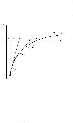
190 Differentiation
approximate values xn and xn+1 are sufficiently close to each other. The question that we still have to discuss is whether specific assumptions have to be made on the initial value x0 in order to ensure that sequence {xn} converges to a zero of function f . The first assumption that we have to make is x0 [a, b] with f (a) · f (b) < 0. In the case of a continuous function, this guarantees that the closed interval [a, b] contains at least one zero x of function f (see Theorem 4.6). However, the latter condition is still not sufficient. It can be proved that, if function f is differentiable on the open interval (a , b ) Df containing [a, b] and if additionally f (x) = 0 and f (x) = 0 for x [a, b] and x0 {a, b} is chosen such that f (x0) · f (x0) > 0, then the above procedure converges to the (unique) zero x [a, b]. The procedure is illustrated in Figure 4.10.
Figure 4.10 Illustration of Newton’s method.
A second possibility is that we approximate function f about x0 by a parabola. This procedure is denoted as Newton’s method of second order. We get:
f (x) ≈ P2(x) = f (x0) + f (x0) · (x − x0) + f (x0) · (x − x0)2. 2!
Let x0 be an initial (approximate) value. Then we obtain from f (x) ≈ P2(x) = 0
f (x0) + f (x0) · (x − x0) + f (x0) · (x − x0)2 = 0. 2!
If we eliminate x and identify it with x1 we get:
|
|
|
|
f (x0) ± |
|
|
. |
x1A,1B |
= |
x0 |
− |
[f (x0)]2 − 2f (x0)f (x0) |
|
||
|
|
||||||
|
|
|
f (x0) |
||||
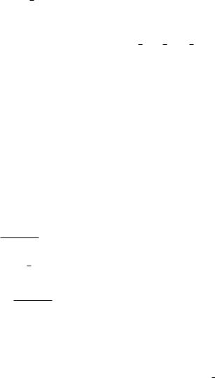
Differentiation 191
Using now x1 = x1A or x1 = x1B (depending on which value is the better approximation of the zero), instead of x0 on the right-hand side of the above equation, we determine a new approximate value x2 and so on. Again some assumptions have to be made to ensure convergence of sequence {xn} to a zero. It can be proved that, if function f is differentiable on the open interval (a , b ) Df containing [a, b] and x0 [a, b] with f (a) · f (b) < 0 and f (x) = 0 for x [a, b], then the sequence {xn} determined by Newton’s method of second order converges to a zero x [a, b].
The above two variants of Newton’s method use derivatives. Finally, we briefly discuss two derivative-free methods for determining zeroes numerically. The first procedure presents a general iterative algorithm, also known as a fixed-point procedure, which transforms the equation f (x) = 0 into the form x = ϕ(x). A solution x with x = ϕ(x) is denoted as fixed-point. Starting with some point x0 [a, b], we compute iteratively the values
xn+1 = ϕ(xn), |
n = 0, 1, . . . . |
The procedure stops when two successive values xk and xk+1 are ‘sufficiently close’ to each other. A sufficient condition to ensure convergence of this approach to a fixed point is that there exists a constant L (0, 1) with
|ϕ (x)| ≤ L |
for all x [a, b]. |
The second derivative-free method is known as regula falsi. In this case, we approximate function f between x0 = a and x1 = b with f (a) · f (b) < 0 by a straight line through the points (a, f (a)) and (b, f (b)). This yields:
y − f (a) = f (b) − f (a) · (x − a). b − a
Since we look for a zero x of function f , we set y = 0 and obtain the approximate value
b − a x2 = a − f (a) · −
f (b) f (a)
for the zero. In general, we have f (x2) = 0. (In the other case, we have found the exact value of the zero.) Now we check which of both closed intervals [a, x2] and [x2, b] contains the zero. If f (a) · f (x2) < 0, then there exists a zero in the interval [a, x2]. We replace b by x2, and determine a new approximate value x3. Otherwise, i.e. if f (x2) · f (b) < 0, then interval [x2, b] contains a zero. In that case, we replace a by x2 and determine then an approximate value x3, too. Continuing in this way, we get a sequence {xn} converging to a zero x [a, b]. This procedure is illustrated in Figure 4.11.
192 Differentiation
Figure 4.11 Illustration of regula falsi.
Example 4.36 Let f : (0, ∞) → R with
f (x) = x − lg x − 3
be given. We determine the zero contained in the closed interval [3, 4] exactly to three decimal places. First we apply Newton’s method. We obtain
f (x) = 1 − |
|
|
|
1 |
|
|
|
|
and |
|
f (x) = |
1 |
|
|
. |
|
|
|
|
||||||
x ln 10 |
|
|
|
|
x2 ln 10 |
and f |
|
|
|
||||||||||||||||
Obviously we have f (3) < 0, f (4) > 0, f (x) > 0 for x |
[ |
3, 4 |
(x) > 0 for x |
[ |
3, 4 . |
||||||||||||||||||||
Using |
|
|
|
|
|
|
|
|
|
|
|
|
|
|
|
|
|
|
] |
|
] |
||||
|
|
|
|
|
|
|
|
|
|
|
|
|
|
|
|
|
|
|
|
|
|
|
|
|
|
x |
x |
|
|
f (xn) |
|
x |
|
xn − lg xn − 3 |
, |
n |
|
0, 1, . . . , |
|
|
|
||||||||||
|
|
|
|
|
|
|
|
|
|
1 |
|
|
|
|
|
||||||||||
n+1 = |
|
n − f |
|
(x |
) |
= |
|
n − |
|
|
|
|
|
= |
|
|
|
|
|
|
|
||||
|
|
|
|
|
n |
|
|
|
|
|
1 |
− xn ln 10 |
|
|
|
|
|
|
|
|
|
||||
we get the results presented in Table 4.2 when starting with x0 = 4. We obtain f (x2) < 10−5, and the value given in the last row in bold face corresponds to the zero rounded to three decimal places.
Table 4.2 Application of Newton’s method
n |
xn |
f (xn) |
f (xn) |
0 |
4 |
0.39794 |
0.89143 |
1 |
3.55359 |
0.00292 |
0.87779 |
2 |
3.55026 |
0.00000 |
|
33.550


Differentiation 195
4.9Given the total cost function C : R+ → R with
C(x) = 4x3 − 2x2 + 4x + 100,
where C(x) denotes the total cost in dependence on the output x. Find the marginal cost at x0 = 2. Compute the change in total cost resulting from an increase in the output from 2 to 2.5 units. Give an approximation of the exact value by using the differential.
4.10Let D : DD → R+ be a demand function, where D( p) is the quantity demand in dependence on the price p. Given D( p) = 320/p, calculate approximately the change
in quantity demand if p changes from 8 to 10 EUR.
4.11 Given the functions f : Df → R+ with
f (x) = 2ex/2
and g : Dg → R+ with
g(x) = 3√x
find the proportional rates of change ρf (x), ρg (x) and the elasticities εf (x) and εg (x) and specify them for x0 = 1 and x1 = 100. For which values x Df are the functions f and g elastic? Give the percentage rate of change of the function value when value x increases by one per cent.
4.12 Given the price–demand function
D = D( p) = 1, 000e−2( p−1)2
with demand D > 0 and price p > 0, find the (point) elasticity of demand εD(p). Check at which prices the demand is elastic.
4.13Find all local extrema, the global maximum and the global minimum of the following functions f : Df → R with Df [−5, 5], where:
(a) f (x) = x4 − 3x3 + x2 − 5; |
(b) |
f (x) = 4 −2 |
|x − 3|; |
||||||||
(c) |
f (x) = e−x2/2; |
(d) |
f (x) = |
x |
|
; |
|||||
x |
2 |
||||||||||
|
|
√ |
|
|
|
|
|
|
− |
|
|
|
x |
|
|
|
|
||||||
(e) |
f (x) = |
1 + √ |
|
. |
|
|
|
|
|
||
x |
|
|
|
|
|
||||||
4.14 Assume that function f : Df → R with
f (x) = a ln x + bx2 + x
has local extrema at point x1 = 1 and at point x2 = 2. What can you conclude about the values of a and b? Check whether they are relative maxima or minima.
196 Differentiation
4.15Determine the following limits by Bernoulli–l’Hospital’s rule:
(a) |
lim |
sin x |
; |
|
|
|
(b) |
lim |
e2(x−1) |
− |
x2 |
||||||
|
|
x |
|
|
|
|
|
2 |
|
2 |
; |
||||||
|
x→0 |
|
|
|
|
|
|
|
|
x→1 (x |
|
− 1) |
|
|
|||
(c) |
lim |
(x2)1/x ; |
|
|
(d) |
lim |
xx ; |
|
|
|
|
||||||
|
x→∞ |
|
|
|
|
|
|
|
x→0+0 |
|
|
|
|
|
|
||
(e) |
lim |
|
|
1 |
|
|
1 |
; (f) |
lim |
1 |
|
|
sin x |
|
|
||
x sin x |
− x2 |
|
ln |
. |
|
||||||||||||
|
x→0 |
|
x→0 x2 |
|
x |
|
|||||||||||
4.16For the following functions f : Df → R, determine and investigate domains, zeroes, discontinuities, monotonicity, extreme points and extreme values, convexity and concavity, inflection points and limits as x tends to ±∞. Graph the functions f with f (x)
given as follows:
(a) |
f (x) |
|
|
x2 |
|
|
1 |
|
; |
|
(b) |
f (x) |
|
|
3x2 |
|
|
|
4x |
; |
||||||
|
|
|
+ |
|
|
|
|
|
|
|
− |
|
||||||||||||||
|
|
|
|
|
|
|
|
2 |
|
|
|
|
|
|
|
|
|
|
|
|
|
|||||
|
|
= (x − 2) |
|
|
|
|
|
|
= |
|
−2x |
2 |
+ x |
|
||||||||||||
|
|
|
|
|
|
|
|
|
|
|
||||||||||||||||
(c) |
f (x) = |
|
|
|
x4 |
+ |
x3 |
; |
(d) |
f (x) = e |
(x |
− |
1)2/2 |
; |
|
|||||||||||
x |
3 |
|
|
2 |
|
|
|
|
|
|
|
|||||||||||||||
|
|
|
|
− 2x |
|
+ x |
|
|
|
|
|
|
|
|
|
|
|
|
|
|||||||
|
|
= |
|
|
|
|
− |
|
|
|
|
|
|
|
|
3 |
|
|
|
|
|
|
|
|||
|
|
|
|
|
|
x |
|
|
|
|
|
|
|
|
= |
|
|
|
− |
|
|
|||||
(e) |
f (x) |
ln |
x |
2 |
2 |
; |
|
(f) |
f (x) |
√2x2 |
x3. |
|||||||||||||||
|
|
|
|
|
|
|||||||||||||||||||||
|
|
|
|
|
|
|
|
|
|
|
|
|
|
|
|
|
|
|
|
|
|
|
|
|
|
|
4.17Expand the following functions f : Df → R into Taylor polynomials with corresponding remainder:
(a) |
f (x) = sin |
π x |
|
= 2, |
n = 5; |
|
|
, |
x0 |
||||
4 |
||||||
(b) |
f (x) = ln(x + 1), |
x0 |
= 0, |
n N; |
||
(c) |
f (x) = e−x sin 2x, |
x0 |
= 0, |
n = 4. |
||
√
4.18Calculate 1/ 5 e by using Taylor polynomials for function f : Df → R with f (x) = ex . The error should be less than 10−6.
4.19 Determine the zero x of function f : Df → R with
f (x) = x3 − 6x + 2 and 0 ≤ x ≤ 1
exactly to four decimal places. Use (a) Newton’s method and (b) regula falsi. 4.20 Find the zero x of function f : Df → R with
f (x) = x − ln x − 3 and x > 1.
Determine the value with an error less than 10−5 and use Newton’s method.