5. Data processing

The results of this laboratory work must be presented in a graphical aspect - is an allocation electric field equipotential lines, the drawing of electric-field vectors in three points. The graphical form of results usually guesses quality estimation and consequently does not demand statistical manipulation.

6. Work execution order and experimental data analysis

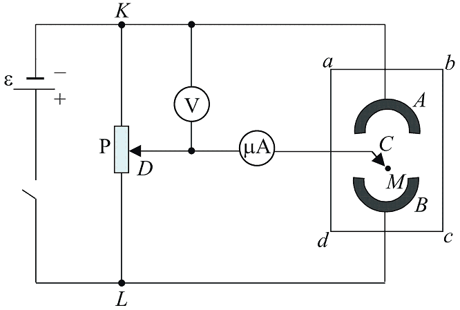
1. Mount the circuit (Fig. 9).

2. With the help of voltmeter measure potential difference U between electrodes A and B by full turning of the handle of potentiometer P.

3. In order to build n equipotential lines divide U on n+1. Take n >5.

4. To outline a pencil on a paper of a surface of electrodes. Obtained lines represent zero ₀=0 and last ₆=U equipotential surfaces.

5. Set on the voltmeter voltage ₁=U/(n+1).

6. By moving the probe C on the paper's surface obtain absence of a current in microampermeter and mark the 8 ̵ 10 points with potential ₁.

7. To join the obtained points a line and to note value of a potential near the gained equipotential line.

8. To set on the voltmeter voltage ₂=2₁ and perform the items 6 and 7.

9. Analogously to build remaining equipotential lines.

10. To calculate an electric intensity in the several points marked by the teacher. For this purpose near to each point by means of a ruler measure a shortest distance between the proximal equipotential lines. By formula to calculate the electric intensity absolute a value. Here =₁ – a potential difference between the neighbouring equipotential lines.

11. To build field lines. On those regions where the absolute value of the electric intensity level gained in item 10 is more, field lines should be placed more densely. To point a direction of field lines.

12. On the absolute values gained in item 10 to build electric-field vectors in scale. Directions of vectors are chosen along tangents to field lines. To mark out the gained vectors.

13. To draw a conclusion about of types of magnitudes, those have been calculated by using of the obtained potential distribution.

7. Test questions

1. What is an electric intensity? What are the units of measurement of the electric intensity? What is the direction of the electric intensity?

2. How to calculate electric intensity of:, an infinite uniformly charged plate, an infinite uniformly charged thread, a point charge?

3. What is the potential of the field in a given point? What are the units of potential?

4. How the work of the electric field forces does defines through the potential difference?

5. What is the field line? Draw the field lines of: positive and negative point charges, plane, and thread.

6. What is equipotential surface? Draw equipotential surfaces of: a plane, a thread, a point charge.

7. What is the relation between intensity and potential?

8. How can in the lab we experimentally find the location of equipotential surfaces?

Draw a scheme.

9. How can we calculate the intensity of the field in point between the equipotential lines?

8. Content of the report

Homework to laboratory work № 2-1

(Answers on test questions from p.14)

…

Laboratory work №2-1 implementation protocol

1) Тopic: STUDYING OF ELECTROSTATIC FIELD

2) Work goal: Study of electrostatic field with the help of equipotential surfaces.

3) Scheme of laboratory research facility:

А и В – set of electrodes, С – probe, Р – potentiometer, V – voltmeter, mА – microamperemeter,  - voltage source, а-в-с-d – cell with conducting paper.

4) Equipment table

№	Name	Type	Serial number	Grid limit	Grid unit	Accuracy class (absolute error)
1.	Volmeter	М 906		5V	0,2V	1,5%
2.	Microampermeter	М 906		50 А	1А	1 %

5) Quantities calculation formulae:

,		where j1 – value of the potential on first equipotential line, when we have obtain of n equipotential lines; U – potential difference between electrodes.
,	where Е – is the absolute value of electric intensity; Dj=j1 – potential difference between the neighboring equipotential lines; –distance between the neighboring equipotential lines between which the value of an electric intensity has to be defined.

6) Table of measurements

№ of piont	, V	, m	E , V/m
1
2
3

7) Quantities calculation:

8) Final result: (Exemplary diagram of distribution of potential and electric field lines)

Experimentally obtained (!!!) diagram (or its copy) with measurements has to be pasted in a protocol.

9) Conclusion: On the experimentally obtained space distribution of a potential we have counted the vectors of … in various points of electric field.

10) Data: “___” _____20___. Work done by: ______ Work checked by:

(Surname, readable)