7) Calculation of quantities:

8) Final results: Plots of dependences of:  - total power PT ,  - useful power PU and  - efficiency η versus load resistance R:

9) Conclusions:

9a) With increasing of load resistance the total power …

9b) With increasing of load resistance the efficiency …

9c) Useful power has a … , when … , therefore optimal mode with greatest delivery to external resistance corresponds to load matching condition … .

10) Data: “___” _____20___. Work done by: ______ Work checked by:

(Surname, readable)

LABORATORY WORK № 3-1

1. Topic: STIDYING MAGNETIC FIELD VIA TANGENT-COMPASS

2. Goal of the work:

2.1. Study of method of a vector diagrams for representation of magnetic field.

2.2. Finding the horizontal component of a magnetic intensity vector in the laboratory via tangent-compass.

3. Main concepts

3.1. Magnetic field of currents. Intensity and induction of magnetic field

Any moving electric charge creates a magnetic field. Electric current (as an ordered motion of charges) creates a magnetic field too. Magnetic field around a permanent magnet is being created by orientation in one direction of atomic micro-currents of material of magnet.

In the magnetic field other moving charge (or current) experiences a force. Thus wires with parallel currents are being attracted and with anti-parallel are being repulsed, because the magnetic field of moving charges of first wire acts on moving charges of the second wire.

As the objects of interaction in magnetism usually consider or moving electric charges or elements of current.

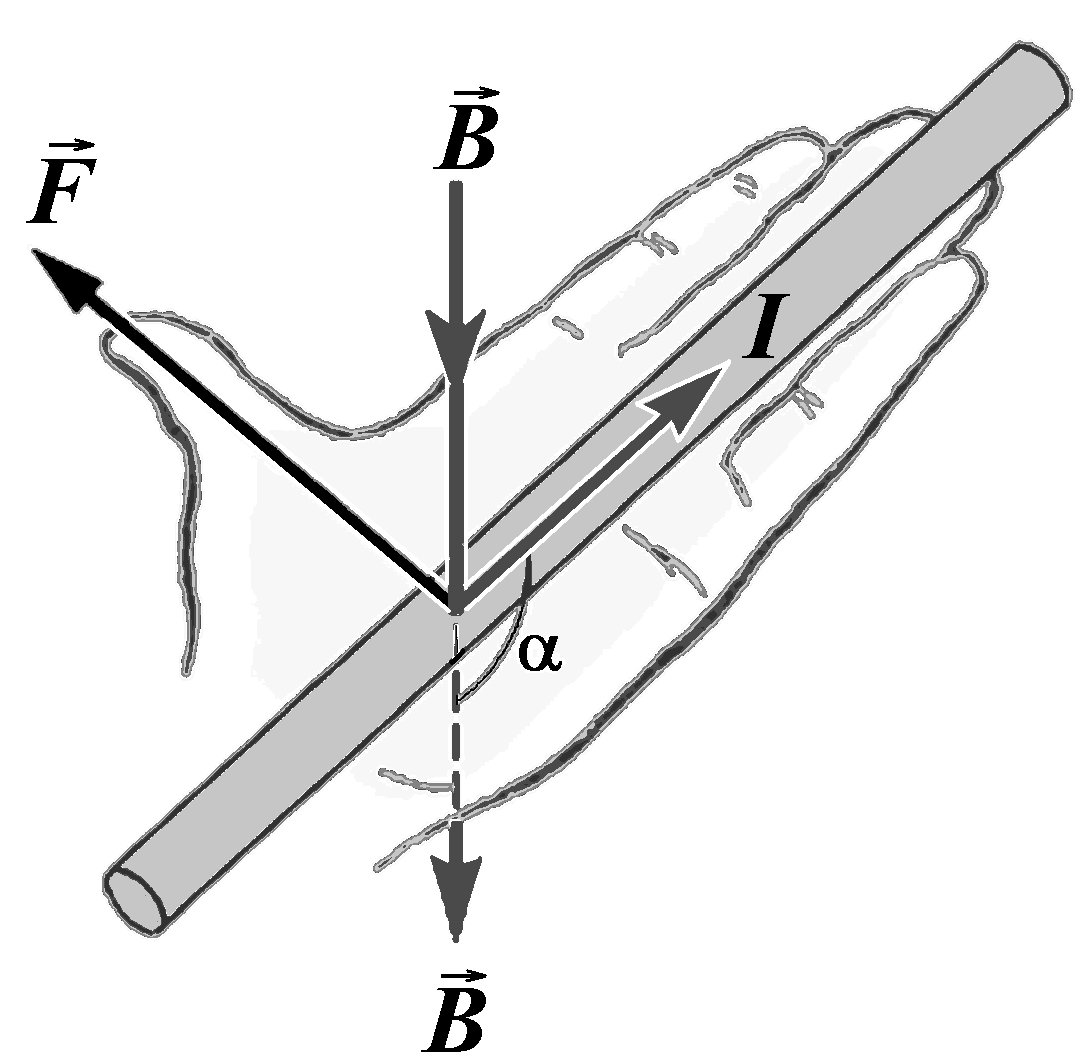
Element of the current Idl – is a product of a current I and infinitesimal segment of wire dl. Element of current is a vector, whose direction coincides with direction of the current. Element of current in Magnetism is similar to test charge in Electrostatics – it is a probe with the help of which we can explore magnetic field. As it has been established by Ampere, any element of the current, placed in a magnetic field B, will experience a force:

, or, in scalars , . (84)

Fig. 23 – Left hand rule

Note that the direction of Ampere’s force doesn’t coincide with that of vector of magnetic induction. Its direction defines by a “left hand rule”: if you place left hand so that four fingers point the direction of current (see Fig. 23), and vector of magnetic induction falls into open palm, then extended thumb points in the direction of Ampere’s force.

Quantity is a vector of magnetic induction. It has same direction as a force, with which magnetic field acts on a north pole of magnetic arrow.

Equation (84) gives us a definition of magnetic induction:

=> ; [B]=T. (85)

Vector of magnetic induction numerically equals to force, with which magnetic field acts on a unit element of current (Idl=1Am), placed perpendicularly to vector of magnetic induction (when ).

Fig. 24 – Corkscrew (right-hand screw) rule

SI unit for is Tesla. Tesla is the induction of such magnetic field which exerts a force of 1N on element of a current of 1 Am, placed perpendicularly to vector

1T = 1N / 1Am.

Graphically magnetic field can be depicted with the help of magnetic field lines (lines of magnetic force). Magnetic field line is a type of line for which the tangent line to the path at each point is parallel to the vector at that point.

In order to determine direction of vector B the corkscrew rule (Fig. 24) is used: if translational motion of screw coincides with current I, then rotational motion point out a direction of magnetic field lines B.

Each element of a current generates a magnetic field around it. Induction of that field defines by Biot-Savart-Laplace law:

, or, in scalars, , (86)

Fig. 25 – Illustration to the

Biot-Savart-Laplace law

here, r – is the distance between the element of a current Idl and the point A at which the field inductionis being computed (Fig. 25);₀=4 ∙10^–7H/m – magnetic constant (permeability of vacuum);  – relative permeability of medium, it shows in what many times induction in a given medium is different from that of vacuum.

Quantity depends on medium, because certain substance magnetizes in external magnetic field and generates certain own magnetic field.

If we divide equation (86) on ₀ we’ll obtain quantity, which is independent from properties of medium – magnetic intensity:

. (87)

Equation (87) is a Biot-Savart-Laplace law for magnetic intensity. It defines the value of magnetic field intensity dH for the field, generated by element of the current Idl. Therefore a definition of magnetic intensity:

. [H]=. (88)

The SI unit for magnetic intensity is ampere per meter.

Directions of andcoincide only in isotropic homogeneous medium or in nonmagnetic material.

If wire has a complex shape (see fig. 25) it can be represented as a huge number of elements of current Idl. Resultant magnetic intensity (or induction) at any point is a vector sum of elementary intensities (or inductions) of fields created by each element of currentIdl individually:

; .

This superposition principle allows determine intensity (or induction) of field, created by wires with different form.

Magnetic intensity characterizes only magnetic field of macroscopic currents, because it don’t depend on magnetic properties of medium. Now, let’s consider some special cases.

3.1.1. Finite segment of current create a circular magnetic field (Fig.26). Magnetic intensity at a distance of r from axis of a current defined with the formula:

, (89)

Fig. 26 – Field lines of segment of a current and corkscrew rule

here r – ₁ and ₂ - angles, which are created radius-vectors, traced from the ends of a conductor to the target point A at which field is being calculated.

Vectors of magnetic intensity and inductionare perpendicular to a plane passing through a segmentBC and point A.

Magnetic field lines are concentric circles around a straight current which are lying in perpendicular plane to a current. Direction of field lines can be determined by the corkscrew rule (Fig. 26): if translational motion of screw coincides with current I, then rotational motion point out a direction of magnetic field lines H.

3.1.2. Infinite straight current create a magnetic field same as a segment (Fig. 27).

If length of a segment (Fig.26) increases then angles α₁ and α₂ will decrease until they become zero as in the case of infinite wire. As cos 0° = 1, then

Н_A = I / 2r. (90)

Fig. 27 – Field lines of an infinite current

Direction of and field lines are the same as for finite segment (Fig.27).

3.1.3. Circular current (single coil) (Fig.28). Magnetic intensity at the center of a circular current can be defined with the formula

Н_C = I / 2R, (91)

Fig. 28 – Field lines of a circular current

here, R – is the radius of a circle. Vector is perpendicular to the plane of a coil in each point underlying in a plane of that coil. It can be derived from superposition principle applied to set of magnetic fields produced by each segment of wiredl separately.

Intensity magnitude on the axis of the circle can be defined with the formula

H_A = IR² / 2(R+h) ^{3 / 2}, (92)

where h – distance from the point in which the field is being calculated to the center of coil.

3.1.4. Solenoid. (Fig.29) is a wire, wound around a cylindrical core. Length of a solenoid is in many times greater than its diameter. Inside the solenoid magnetic field there is uniform with intensity

H = IN / l = In, (93)

Fig. 29 – Field lines of solenoid

where, N - number of loops of wire in a solenoid, l – solenoids length, n – number of loops per unit length(winding density). Uniformity of a field is broken at ends of solenoid. Outside there is a weak field with respect to an inside field. Direction of field lines can be defined in the same way as in the case of single coil.

Fig. 30 – Torus

3.1.5. Torus (Fig. 30) is a wire wound around a toroidal core. Torus has no boundary effect. Magnetic field is completely concentrated inside the torus, field lines are concentric circles. If the diameter of loopsD is in many times smaller than the length of torus circle, the intensity can be defined with the formula (50):

Н = IN / l = Iп, (93)