

3.1. Ohm’s law for various circuit units
From (54), (55), (57) and (58) let's write down Ohm's law for these four cases: - for nonuniform electric circuit unit 1-2 consisting only one source of the EMF (see fig. 13)
![]() ;
(59)
;
(59)
- for nonuniform circuit unit 1-3, which contains the source and an external (load) resistor R (see Fig. 14)
![]() ;
(60)
;
(60)
- for closed electric circuit (see Fig. 16)
![]() ;
(61)
;
(61)
- for uniform circuit unit 2-3 consisting only external (load) resistor R (see Fig. 14, 15 and 16)
![]() .
(62)
.
(62)
Using the Ohm’s law we can solve only nonbranched circuits or circuit units. For a solution of branched circuits it is used Kirchhoff rules (23) - (24).
4. Description of laboratory research facility and methodology of measurements
Devices and accessories (Fig: 17, а): Two sources of EMF e1 – modelling source and e2 – auxiliary source, voltmeter V, microamperemeter mA (null the indicator with null in the middle of a dial), potentiometer P, one-decade resistors box R2, switches K1 и K2.
As a modelling source of the EMF with the unknown value of EMF, we choose a source e1. In series with it we connect one-decade resistors box R2 which will model an internal resistance of this source. Thus, we obtain a modelling source of the EMF with a variable internal resistance:
Х=1; rX=r1+R2. (63)
4.1. Measurement of emf of a source with the compensation method
If we connect the voltmeter (Fig. 18) directly to the terminals of a current source, then it will not show us the EMF of source. Voltmeter shows the potential difference, or the voltage between the points A and B, to which it is connected.
As it was shown earlier (54)
UVDIR=B–A=Х–IrХ. (64)
Compensation method is being based on a fact that the potential difference on the poles of the source equals EMF, if the current in the source is absent I=0. We can get this by auxiliary source, which is switched towards the first, as it is shown in Fig. 17,a. The requirement e2>e1 should be satisfied for the full compensation of a current.
If we close the switch К1, when the switch К2 is open, then current will flows through the circuit K2MDCe2. On the circuit unit K1LDCBe1A current is absent. So, potentials of points B and C are the same jC–jВ (see bottom part of Fig. 17,a). At open-circuit mode the potential of the point A is greater than potential of the point B on the quantity eX : jА–jВ=eХ (see bottom part of Fig. 17,a). If jМ–jС>eХ, then jМ>jA>jС, that's why we can always find such point F on potentiometer, which potential jF=jA is equal to potential of the point А (see bottom part of Fig. 17,b).
|
|
|
|
|
|
|
a) |
b) | |||
|
Fig. 17 – The compensation method scheme: а) switch К1 open, а) switch К1 closed
| ||||
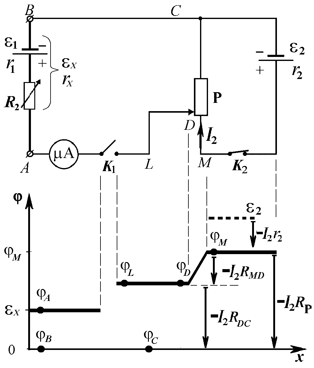
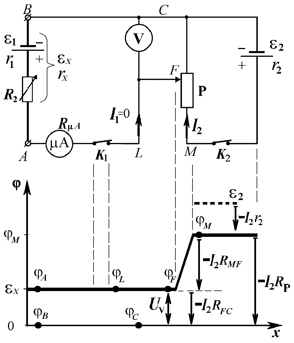
If we put potentiometer slider into the such point F and close the switch К2, then current on the circuit unit AF won’t flow, as jА–jF=0. Current won’t flow through the circuit units AB and BC, which are in-series with the part AD. We say that at this case, the voltage eХ is being compensated by voltage of auxiliary source e2. Microampermeter scale indication is equal zero І1=0.
If the potentiometer slider is situated in point D (as on Fig. 17,a) and switch К1 is closed, then through the circuit unit DABC a current I1 will flow. In this case voltage on circuit unit terminals DC similarly (55):
Let's write voltage 1-3 CBAD:
D –C=Х –I1(RA+rX). (65)
If the potentiometer slider is situated in point F (as on Fig. 17,b), then І1=0:
F–C=Х.
We connect the voltmeter V between points C and F for measuring this value (as shown on the Fig. 17,b). In this case value of internal resistance of the voltmetre does not influence for instrumentation indications as in (64), such as from (65) it is visible, if І =0 we always obtain
UVCOMP=jF –jC=eХ.
Conclusion: total error of measurements of EMF by compensation method eХ=UV is equal only to the voltmeter's error.