Hysteresis

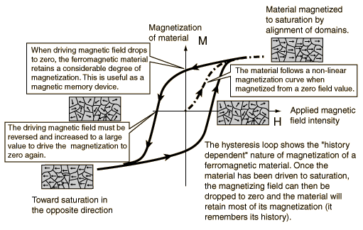
When a ferromagnetic material is magnetized in one direction, it will not relax back to zero magnetization when the imposed magnetizing field is removed. It must be driven back to zero by a field in the opposite direction. If an alternating magnetic field is applied to the material, its magnetization will trace out a loop called a hysteresis loop. The lack of retraceability of the magnetization curve is the property called hysteresis and it is related to the existence of magnetic domains in the material. Once the magnetic domains are reoriented, it takes some energy to turn them back again. This property of ferrromagnetic materials is useful as a magnetic "memory". Some compositions of ferromagnetic materials will retain an imposed magnetization indefinitely and are useful as "permanent magnets". The magnetic memory aspects of iron and chromium oxides make them useful in audio tape recording and for the magnetic storage of data on computer disks.

Hysteresis loop

Area of hysteresis loop is equal to work required to re-magnetize the ferromagnet.

Variations in Hysteresis Curves

Coercivity and Remanence in Permanent Magnets

Agood permanent magnet should produce a high magnetic field with a low mass, and should be stable against the influences which would demagnetize it. The desirable properties of such magnets are typically stated in terms of theremanence and coercivity of the magnet materials.

Description of laboratory research facility and methodology of measurements

Magnetic properties of ferromagnetics are investigated in this work. In order to do this the circular core, made from investigated material, is winded by two coils: primary, with the number of winds N1 and secondary, with N2, which are switched in a circuit as it’s shown in a protocol below, where: T – torus; N1 – primary coil; N2 – secondary coil; P – potentiometer; mA – miliamperemeter; C – capacitor; R1 and R2 – resistors with known resistance; ЭO – cathode-ray oscilloscope.

In order to obtain a hysteresis loop on oscilloscope screen the voltage proportional to the magnitude of induction B should be applied to vertical plates (y - terminals) of cathode-ray tube and voltage proportional to the magnitude of intensity H - to horizontal plates (x - terminals).

Let us prove that the voltage on a resistor R1 in a primary coil circuit is proportional to H and voltage on a capacitor C is proportional to B.

There is alternating current i from external source in a primary coil circuit. Magnetic field intensity in a torus is:

H = i1n1,

where n1 – is number of coils of primary coil per unit length of a torus.

The voltage on a resistance R1 is :

U1 = i1R1.

Considering i1 = Н / п1, obtain

(1)

This voltage is applied to horizontal plates of oscilloscope.

The alternating current in a primary coil causes appearance of induced EMF in a secondary coil, which is proportional to rate of change of magnetic flux:

.

The magnetic flux, piercing cross-sectional area of a torus is:

Ф = ВS.

Hence,

.

This EMF will cause the appearance of a current in secondary coil circuit:

.

The resistance of secondary coil circuit might be taken R2, as long the resistance of capacitor is rather small, with respect to R2. The voltage on a capacitor:

.

Now we put the value of i2 in equation for Uc and evaluate it:

.

This voltage is proportional to magnetic field induction B. It is applied to vertical plates of oscilloscope.

(2)

Thus, the deviation of cathode ray trace on a screen of oscilloscope is proportional to H on horizontal, and to B on vertical. It will trace B = f(H) – curve 50 times per second because the frequency of a current is 50 Hz. The limits in which H changes, can be changed by changing the amplitude of i1 in a primary coil.

The main hysteresis loop will appear when the limits of change of H is such that the ferromagnetic magnetize till saturation; the secondary loops will appear in opposite case. Peaks of all secondary loops lies on main magnetization curve. Hence, in order to obtain main magnetization curve the coordinates nx and ny of secondary loops peaks has to be measured.

By knowing the voltages ux and uy, which rejects the ray on one scale grid, the magnitudes of voltages Ux and Uy can be defined:

Ux = nxиx,

Uy = nyиy.

Magnitude of H can be defined from (1) as:

.

п1, R1, r stay permanent during this work, its magnitudes is on apparatus, so the last equation can be evaluated as:

H = kxnx

(3)

where .

Equation for induction B we’ll obtain from (2):

,

or .

(4)

where

(5)

kx and ky has to be calculated on known initial data before measurements.

Experimental task for this work is to plot magnetization curve (B vs H) and µ vs H curve.

In order to do this we use oscilloscope with image of hysteresis loop on its screen and potentiometer. By decreasing current with the help of potentiometer form maxim value to minimum we measure coordinates nx and ny of vertices of obtained hysteresis loops. Then, by equations (3) and (4) calculate B and H. Calculating permeability as we plot B and µ vs H dependencies on one graphic.