

500 |
|
SEQUENCE-SPECIFIC MANIPULATION OF DNA |
|
|
|
|
|
|
|
|
|
|
|
||||||
than the true target, the ratio of true target to mimic products can be determined. These |
|||||||||||||||||||
approaches |
fall |
far |
short |
of the mark |
when the goal |
is |
to |
analyze many |
genes |
of |
interest. |
||||||||
A number of interesting methods have been developed to sample mRNAs or correspond- |
|
||||||||||||||||||
ing cDNAs and look for expression differences or patterns in biological states. These are |
|||||||||||||||||||
still evolving rapidly. |
|
|
|
|
|
|
|
|
|
|
|
|
|
|
|
||||
In differential display a degenerate short PCR primer is used to amplify the cellular |
|||||||||||||||||||
population of cDNAs. This can be a poly dT complementary to the 3 |
|
|
|
|
|
|
poly A sequence of |
||||||||||||
messages, it can be an anchored dT |
|
|
|
n |
(Liang |
et |
al., |
1994), a short oligonucleotide, or a |
|||||||||||
short sequence complementary to the end of DNA fragments generated by type II-S re- |
|||||||||||||||||||
striction enzymecleavage (Kato, 1995). Type II-S enzymes cut outside of their recogni- |
|||||||||||||||||||
tion sequences to yield a mixture of different single-stranded overhangs. A subset of this |
|||||||||||||||||||
mixture can be captured by ligation to complementary |
overhangs, |
a technique |
that |
has |
|||||||||||||||
been called molecular indexing (Unrau and Deugau, 1994). Regardless of the method |
|||||||||||||||||||
used, the result is to reduce the complexity of the mRNA population and amplify the re- |
|||||||||||||||||||
sulting cDNA to produce a discrete set of species to analyze quantitatively. The analysis |
|||||||||||||||||||
can be performed by conventional or fluorescence-detected gel electrophoresis, or by hy- |
|||||||||||||||||||
bridization (or two-color competitive hybridization) to an array of DNA probes analogous |
|||||||||||||||||||
to the arrays used for SBH (Chapter 12). |
|
|
|
|
|
|
|
|
|
|
|
|
|||||||
These differential display methods are extremely |
powerful |
and |
broadly |
applicable. |
|||||||||||||||
They suffer from a common limitation that whenever PCR amplification must be applied |
|||||||||||||||||||
to a complex sample, the actual population of preexisting mRNAs will be distorted by |
|||||||||||||||||||
differences in their ability to sustain multiple rounds of amplification. Two very different |
|||||||||||||||||||
approaches for avoiding PCR-induced distortions are |
actively |
being |
explored. Picking |
||||||||||||||||
cDNA clones at random and identifying them after sequencing is a |
powerful but |
expen- |
|||||||||||||||||
sive method. Alternatively, cDNAs can be sampled prior to amplification by cutting out a |
|||||||||||||||||||
specific short fragment. The fragments are co-ligated into concatemers and amplified as a |
|||||||||||||||||||
group. Then sequencing of cloned concatemers reveals relative abundances in a clever ap- |
|||||||||||||||||||
proach termed serial analyses of gene expression (SAGE). |
|
|
|
|
|
|
|
|
|
||||||||||
An alternative to differential display is differential cloning. Differential cDNA cloning |
|||||||||||||||||||
can proceed by schemes very similar to the one shown in Figure 14.25, or they |
can in- |
||||||||||||||||||
volve more |
elaborate techniques such as illustrated |
for |
the |
preparation |
of |
normalized |
|||||||||||||
cDNA libraries in Chapter 11. The objective is to recover cDNAs that represent messages |
|||||||||||||||||||
present in one cell type but not another. The more carefully the cell types are selected, to |
|||||||||||||||||||
differ just in the desired characteristics, the more efficient will be the search for the genes |
|||||||||||||||||||
responsible for those characteristics. Differential cDNA cloning can be used to prepare |
|||||||||||||||||||
genes specific for particular tissue types, developmental stages, |
chromosome |
origin, or |
|||||||||||||||||
even subchromosomal origin. These procedures are particularly effective when the target |
|||||||||||||||||||
differences are very small and precisely defined. Examples are differences between unac- |
|||||||||||||||||||
tivated and activated lymphocytes, to recover specific immune response genes, or differ- |
|||||||||||||||||||
ences between regenerating and nonregenerating tissue to |
isolate |
specific |
growth |
factors. |
|||||||||||||||
As in genomic subtractive cDNA cloning, PCR can be used very effectively to solve most |
|||||||||||||||||||
problems |
caused |
by |
small |
samples |
or |
rare messages. |
In |
|
principle, |
PCR |
should |
allow |
|||||||
cDNAs to be made and subtracted from targets as small as single cells. |
|
|
|
|
|
|
|||||||||||||
COINCIDENCE |
CLONING |
|
|
|
|
|
|
|
|
|
|
|
|
|
|
|
|
||
Subtractive cloning allows the selective isolation of DNAs that differ in two samples. A |
|||||||||||||||||||
related, |
but technically |
somewhat |
more demanding |
approach |
is |
coincidence |
amplifica- |
||||||||||||
COINCIDENCE CLONING |
501 |
tion, involving either cloning or PCR, which is designed to allow the selective isolation of DNAs that are the same in two samples. In contrast to subtractive hybridization, which tries to purify unique homoduplexes (i.e., unique differences between samples), coincidence amplification targets unique similarities or homoduplexes between samples. Coincidence amplification will be most useful when two samples are available that con-
tain only a small amount of DNA in common. A number of such situations exist. For example, suppose that one has isolated a chromosome or just a fragment of a chromosome in a hybrid cell. A successful coincidence cloning procedure would allow one to clone out just the human component by using DNA from normal human cells as the second sample.
Two hybrids that contain only a |
small overlap |
region on a single human chromosome |
could allow the selective cloning |
of just that |
overlap region. Large DNA fragments cut |
out from a PFG fractionation could be used in coincidence cloning experiments with hybrid cell DNA to purify human components that lie, specifically, on a pre-chosen fragment size. Finally large DNA fragments could be used in coincidence with other large fragments to selectively clone just regions of overlap. Alternate PCR procedures exploiting human-specific interspersed repeating sequences may be used to isolate the human
specific |
DNA. We will describe |
these methods in detail later in this chapter. |
However, |
they are not as general or as powerful, in principle, as coincidence cloning. |
|
||
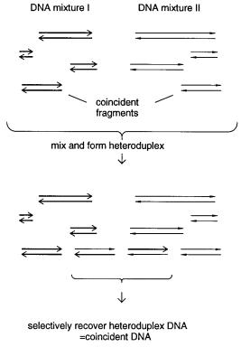
The |
basic task that has to |
be accomplished in any coincidence amplification |
is shown |
in Figure 14.29. DNAs from the two samples to be tested are melted, mixed, and allowed to reanneal. Most fragments in the samples will form homoduplexes because most of the
DNA in two well-chosen samples will be different. Occasional heteroduplexes will be
Figure 14.29 Basic requirements for coincidence cloning or coincidence PCR.

502 |
|
SEQUENCE-SPECIFIC MANIPULATION OF DNA |
|
|
|
|
|
||
formed when sequences in the two samples match very accurately. What is needed, then, |
|
||||||||
is a |
way |
of specifically cloning or amplifying the heteroduplexes. Note that |
this |
is a |
|||||
different |
problem than the heteroduplex detection we described in Chapter 13. In that |
||||||||
case |
the |
desired heteroduplexes |
were |
those with |
one or |
more |
mismatches, |
and |
the |
mismatches |
were used as a specific |
handle |
to detect or |
capture |
the |
heteroduplexes. |
Here |
|
|
the desired heteroduplexes will in general |
be perfect matches. Quite a |
few |
different |
|||
schemes have been tested for coincidence cloning (Box 14.3). None |
appear to |
work |
||||
totally satisfactorily yet. |
|
|
|
|
|
|
|
|
|
|
|
|
|
BOX 14.3 |
|
|
|
|
|
|
PROPOSED SCHEMES FOR COINCIDENCE AMPLIFICATION |
|
|
|
|
|
|
Although these schemes for coincidence cloning are |
largely |
unproved, we |
will |
de- |
|
|
scribe them in some detail because they |
illustrate |
some of |
the available arsenal |
of |
||
tricks for manipulating DNA sequences (Brooks and Porters, 1992). Similar schemes can be conceived of for coincidence PCR (Barley et al., 1993).
Figure 14.30 A scheme for coincidence cloning based on preferential cleavage of methylated homoduplexes. Adapted from Brooks and Porteus (1992).
(continued)

|
|
|
|
|
|
|
|
|
|
|
|
|
|
|
|
|
|
|
|
|
|
COINCIDENCE |
CLONING |
|
503 |
|
BOX 14.3 |
|
(Continued) |
|
|
|
|
|
|
|
|
|
|
|
|
|
|
|
|
|
|
|
|
|
|||
|
Figure 14.30 shows a scheme for differential cloning |
of |
heteroduplexes |
based on |
|
|
|
|||||||||||||||||||
DNA methylation and the unusual properties of restriction enzymes |
like |
|
|
|
|
|
|
|
Dpn |
I. This |
|
|||||||||||||||
enzyme has already been described in Chapter 8, where it was used to |
generate |
large |
|
|
|
|
||||||||||||||||||||
DNA fragments by selective cutting. Here it will be used to destroy homoduplexes se- |
|
|
|
|
|
|||||||||||||||||||||
lectively. The scheme in Figure 14.30 requires two different restriction enzymes with |
|
|
|
|||||||||||||||||||||||
the |
ability, |
like |
Dpn |
|
I, |
to cut |
only |
fully |
methylated |
DNA duplexes. DNA from one |
|
|
|
|||||||||||||
sample is methylated with one conjugate methylase; the second conjugate methylase is |
|
|
|
|
|
|||||||||||||||||||||
used to methylate DNA from the second sample. Then the two samples are mixed, de- |
|
|
|
|
|
|
||||||||||||||||||||
natured, and allowed to renature. The key feature of the resulting mixture is that all |
|
|
|
|
||||||||||||||||||||||
homoduplexes |
will |
|
be fully methylated at their respective sites, and |
they |
will |
|
be |
cut |
|
|
|
|
||||||||||||||
into small pieces when treated with a mixture of the two corresponding restriction |
|
|
|
|
||||||||||||||||||||||
nucleases. Only |
|
heteroduplexes will be hemi-methylated |
at all of |
the |
restriction |
sites |
|
|
|
|
||||||||||||||||
in question, and so they should be much less sensitive targets for cleavage. Thus a size |
|
|
|
|
||||||||||||||||||||||
fractionation after the digestion should allow the preferential isolation and subsequent |
|
|
|
|
||||||||||||||||||||||
cloning or PCR of the heteroduplexes. The flaw in this scheme, as |
in |
the |
|
|
|
Dpn |
I- |
|||||||||||||||||||
mediated specific DNA cleavage discussed in Chapter 8, is that it |
requires |
nucleases |
|
|
|
|
||||||||||||||||||||
that |
do |
not |
cut |
|
hemi-methylated |
DNA. |
|
|
|
|
Dpn |
|
|
I |
at least |
does |
not have |
this necessary |
|
|
||||||
property. |
|
|
|
|
|
|
|
|
|
|
|
|
|
|
|
|
|
|
|
|
|
|
|
|
|
|
|
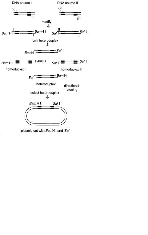
A second scheme for coincidence cloning |
|
is illustrated |
in |
Figure |
14.31. |
This |
|
|
|
||||||||||||||||
scheme is based on the frequently used method of directional cloning. A vector is em- |
|
|
|
|
|
|||||||||||||||||||||
ployed that requires two different ligatable ends for efficient cloning of a target. DNA |
|
|
|
|
||||||||||||||||||||||
from one source is amplified with a PCR primer |
with an extension that generates |
one |
|
|
|
|
||||||||||||||||||||
of the necessary ends. DNA from the second source is amplified with the same PCR |
|
|
|
|
|
|||||||||||||||||||||
primer with an extension having different restriction enzyme cleavage |
sites. The best |
|
|
|
|
|||||||||||||||||||||
way to do this would be to start with separate libraries of the two source DNAs in the |
|
|
|
|
||||||||||||||||||||||
same vector. In this way tagged single primers corresponding to flanking vector se- |
|
|
|
|
||||||||||||||||||||||
quence could |
be |
|
used for efficient PCR. Alternatively, tagged |
random |
primers |
or |
|
|
|
|
||||||||||||||||
tagged short specific primers could be used (see Chapter 4). This is a more general ap- |
|
|
|
|
||||||||||||||||||||||
proach that could be applied directly to genomic DNA, but it is likely to be much less |
|
|
|
|
||||||||||||||||||||||
efficient. |
After |
amplification |
the |
samples |
are |
treated |
with |
the |
|
restriction |
|
enzymes |
|
|
|
|
||||||||||
needed to cleave within the sites introduced by the primer extensions. Then the two |
|
|
|
|
||||||||||||||||||||||
samples are melted, mixed, and reannealed. In principle, only heteroduplexes will have |
|
|
|
|
|
|||||||||||||||||||||
the necessary ends required for efficient directional cloning. |
|
|
|
|
|
|
|
|
|
|
|
|
|
|
||||||||||||
|
In practice, this approach is likely to have problems of low yield and significant |
|
|
|
|
|||||||||||||||||||||
contamination with unwanted homoduplexes. Unless all of the cloned DNA is dephos- |
|
|
|
|
|
|
|
|||||||||||||||||||
phorylated, |
it |
will be quite common to co-clone homoduplex |
and |
heteroduplex |
|
|
|
|
||||||||||||||||||
fragments. Since the former are present in vast excess, they will contaminate most |
|
|
|
|
||||||||||||||||||||||
samples. |
Even if |
|
the restriction |
fragments |
are |
|
dephosphorylated |
prior |
to |
ligation |
to |
|
|
|
|
|||||||||||
the vector arms, homoduplexes will be the major initial ligation product with the vast |
|
|
|
|
||||||||||||||||||||||
majority of the vector. This will consume most of the vector, and although the subse- |
|
|
|
|
||||||||||||||||||||||
quent cloning of the resulting linear products will be relatively inefficient, it is likely to |
|
|
|
|
||||||||||||||||||||||
occur often enough to lead to a very serious background of unwanted homoduplex |
|
|
|
|
|
|||||||||||||||||||||
products. |
|
|
|
|
|
|
|
|
|
|
|
|
|
|
|
|
|
|
|
|
|
|
|
|
|
|
|
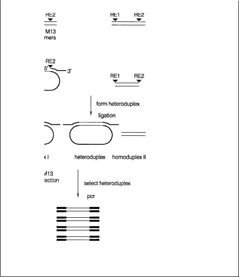
A third strategy for coincidence cloning is presented in Figure 14.32. This appears |
|
|
|
||||||||||||||||||||||
to be potentially powerful, but it is also fairly complex. DNAs from two sources are |
|
|
|
|
||||||||||||||||||||||
separately treated |
with the |
same |
two |
restriction |
enzymes to |
form |
mixture |
of |
double |
|
|
|
|
|||||||||||||
(continued)
504 SEQUENCE-SPECIFIC MANIPULATION OF DNA
BOX 14.3 |
(Continued) |
|
|
|
|
|
|
|
Figure 14.31 A scheme for coincidence cloning based on preparation of heteroduplexes to facilitate directed cloning. Adapted from Brooks and Porteus (1992).
digest products. One of the samples is left as restriction fragments. The other is directionally subcloned into the bacteriophage vector M13. Double-stranded flanking vector sequences, containing additional DNA segments, that will subsequently be used for PCR, are annealed to DNA from the M13 clones. Then both samples are melted, mixed, and allowed to reanneal. Heteroduplexes will be formed when restriction frag-
ments from the first sample match clones from the second sample exactly. These are ligated to the tagged vector arms. Then PCR is used, with primers corresponding to the tagged sequences, to amplify the heteroduplexes specifically. The samples will be contaminated at this point by large amounts of M13 clones, but since these are all significantly larger than the PCR products, it should be possible to remove them by size selection.
(continued)
COINCIDENCE CLONING |
505 |
BOX 14.3 |
(Continued) |
Figure 14.32 A scheme for coincidence cloning based on preparation of a complex that allows selective PCR of heteroduplexes. Adapted from Brooks and Porteus (1992).
There would be many interesting applications of robust coincidence cloning amplification procedures. For example, coincidence cloning of a cDNA library and a YAC should
allow efficient capture of all of the genes on the YAC in a single step. Coincidence cloning of cDNAs from two very different tissue types should result in a highly enriched population of housekeeping genes that are not tissue specific. Finally coincidence cloning
could be a very effective way to isolate very specific human DNAs from hybrid cell lines.
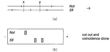
An example of this is shown in Figure 14.33. Here probes of interest detect PFG-fraction- ated large human restriction fragments in a rodent background, and the goal is to obtain clones for the human DNAs contained on these fragments. The key point is that the hu-
man DNAs recognized by the same probes in the two different digests must have corresponding DNA sequences, while the rodent DNA that contaminates each human fraction
506 SEQUENCE-SPECIFIC MANIPULATION OF DNA
Figure 14.33 |
|
How coincidence cloning might be used to enrich the DNA from particular large |
re- |
||
striction |
fragments |
seen |
by hybridization in rodent-human hybrid cells. |
|
(a) Restriction map of the |
region; |
X and |
Y |
indicate two human-specific probes. |
(b) Southern |
blot of a PFG fractionation hy- |
bridized |
with the |
two available probes. Intact material from a duplicate |
PFG run would be used to |
||
cut out the regions detected by hybridization, and one digest would be used in coincidence cloning with the other.
is likely to be different. Thus coincidence cloning of DNAs from a pair of gel slices from the two different digests should preferentially yield the human material. Even more complex logical cloning schemes consisting of various separation and amplification steps can
be conceived of. Their ultimate utility will depend on how effective the more simple straightforward procedures become.
HUMAN INTERSPERSED REPEATED DNA SEQUENCES |
|
|
|
Most repeated sequence DNA in the human genome and other complex genomes appears |
|
||
to be interspersed with single-copy |
DNA. Although plenty of tandem repeats |
exist, such |
|
as VNTRs, except for centromeres these actually make up only a small |
fraction of |
the |
|
class of highly repeated sequences. The original demonstration that the bulk of the human |
|
||
repeats was interspersed was done |
in a series of classic experiments |
by Britten |
and |
Davidson. Subsequently the type of analysis they used has been refined and elaborated by
Robert Moyzis and his colleagues. The basic scheme that underlies these approaches is
shown in Figure 14.34 |
a . A trace amount of labeled total human DNA is sheared randomly |
||
to various average lengths, |
|
L . This DNA is hybridized in solution with a vast excess of |
|
much shorter driver DNA. The driver DNA consists of unlabeled total human DNA iso- |
|||
lated as all of the duplex that |
forms at |
a |
C 0 t of less than or equal to 50. This sample will |
contain all significant high-copy number human repeats but will contain very little single- |
|||
copy DNA or infrequent repeats such as those seen in gene families. The hybridization of |
|||
the driver with the labeled DNA is carried out at a |
C 0 t of 12.5. The goal of the experiment |
||
is to determine how much of the total labeled DNA can be captured by the repeated DNA |
|||
driver during the hybridization. |
|
|
|
The basic idea behind the experiment in Figure 14.34 |
a is that all the DNA in clustered |
||
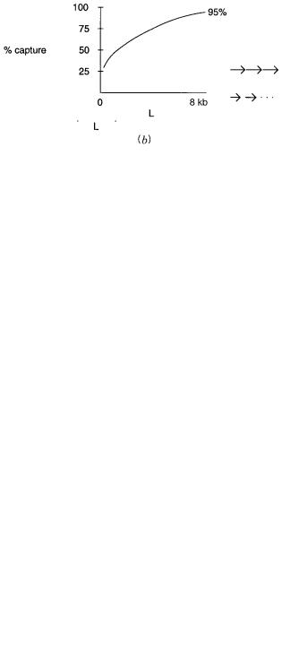
repeats will be captured very easily and efficiently, regardless of the length of DNA target |
|||
used. In contrast, when |
L |
is small, most interspersed DNA will be captured without flank- |
|
ing single-copy sequences. As |
|
L increases, |
more and more single-copy DNA will be cap- |
HUMAN INTERSPERSED REPEATED DNA SEQUENCES |
507 |
Figure 14.34 |
Analysis of |
the pattern of repeats in |
human |
DNA by |
renaturation kinetics. |
(a) |
Design of the basic experiment. Purified repeat is used in excess |
as the |
driver |
to capture indexed |
|
||
genomic DNA fragments of length |
L . (b) Two possible extreme patterns of repeating sequence. |
|
||||
tured by virtue of its neighboring repeated DNA (Figure 14.34 |
|
|
|
|
b ). A typical experimental |
||
result from such a procedure is shown in Figure 14.35. It is evident |
that |
only |
about a |
||||
quarter of the genome is captured when |
L |
is small; |
this provides an estimate for the total |
||||
amount of highly repeated DNA. Almost all of the genome is captured by the time the av- |
|
|
|
||||
erage fragment size reaches 8 kb. Thus |
many single-copy DNAs have a |
repeated |
se- |
|
|||
quence within 1 kb, and almost all single-copy DNAs have a repeat within 8 kb. The sim- |
|
||||||
plest fit to the data in Figure 14.35 |
suggests the occurrence of an |
interspersed |
repeat |
||||
every 3 kb. A more elaborate and more accurate fitting procedure suggests that the distri- |
|
||||||
bution of repeats is bimodal. About 58% |
of the genome has a |
repeat on |
average |
every |
|
||
1 kb; the remainder of the genome has a repeat on average every 8 kb. Of course this |
|||||||
analysis does not reveal any information about the nature of the repeats or the number of |
|
||||||
different basic kinds of repeats and their particular distribution. |
|
|
|
|
|
|
|
In fact there are just a few known major types of interspersed repeats in the |
human |
||||||
genome. Their properties are summarized in Table 14.3. By far the most common human |
|
||||||
repeat is a sequence called Alu because it contains two cutting sites for the restriction en- |
|||||||
zyme Alu I. Thus when human DNA is cut with Alu I and fractionated by size, the result- |
|
||||||
ing material shows a bright, specific size |
band standing out from a background |
broad |
|
||||
smear of other fragment sizes. There may be as many as 10 |
|
|
|
|
|
6 Alu sequences in the human |
|
genome. Very similar sequences are seen in other primates, but in more diverged species, |
|
||||||
like rodents, the Alu-like sequences are sufficiently different |
that Alu’s |
can be |
used |
as |
|||
Figure 14.35 Fraction of total genomic DNA captured at low C
ver, as a function of the length, |
L , of the genomic DNA used. Adapted from Moyzis et al. (1989). |
508 |
SEQUENCE-SPECIFIC MANIPULATION OF DNA |
|
|
|
|
|
|||
TABLE 14.3 |
Major Known Human Repeats |
|
|
|
|
|
|
||
|
|
|
|
|
|
|
|
|
|
|
|
|
|
Hybridization |
|
GenBank |
|
|
|
|
|
Abundance |
Average |
Average |
Average |
Total Mass |
|
||
Type |
|
(Copies) |
Spacing |
|
Spacing |
Length |
(Est.) |
|
|
|
|
|
|
|
|
|
|
||
3 line (L1) |
5 |
104 – 105 |
30 – 60 kb |
|
27 kb |
1.1 kb |
55 – 110 Mb |
||
Intact L1 |
|
4 |
103– 104 |
150 – 480 kb |
|
|
— |
6.4 kb |
Trivial |
(GT) |
|
5 |
104 – 105 |
30 – 60 kb |
|
54 kb |
0.04 kb |
Trivial |
|
n |
|
|
105 – 106 |
|
|
|
|
|
|
Alu |
|
5 |
3–6 kb |
|
|
4 kb |
0.24 kb |
120 – 240 Mb |
|
general species-specific DNA probes. A typical Alu sequence is around 0.24 kb and actually consists of an approximate tandem repeat of a shorter sequence. This is illustrated in Figure 14.36, which shows the consensus among known Alu sequences. Alu is an example of a class of repeating DNA sequences called short interspersed repeat sequences (SINES). Alu sequences in the human are far from identical. Known sequences have been classified into at least five different families, and even within a family the average difference between two Alu’s is roughly 10%.
HS CON |
G |
G |
C |
C |
G |
G |
G |
C |
GC |
|
G |
G |
T |
G |
G |
C |
T |
C |
AC |
G |
C |
C |
T |
G |
T |
A |
A TC |
C |
C A |
G C A C |
T TT |
G G |
G |
A G G |
C |
C |
GA |
50 |
pPD39 |
. |
. |
. |
. |
. |
. |
. |
. |
. |
. |
. . . . . . . . . . |
. . . . . . . . . . |
. . . . . . . . . . |
. . . . . . . . . . |
||||||||||||||||||||||||
BLUR 8 |
X |
X |
X |
X |
X |
X |
X |
X |
X |
X |
X |
X |
X |
X |
X |
X |
X |
X |
X X |
X |
X |
X |
X |
. |
. |
. |
. . . |
. . . . . . . . . . |
. . . . . . . . A . |
|||||||||
HS CON |
G |
G |
C |
G |
G |
G |
C |
G |
GA |
|
T |
C |
A |
C |
G |
A |
G |
G |
TC |
A |
G |
G |
A |
G |
A |
T |
C GA |
G |
A C |
C A T C |
C CC |
C C |
T |
A A A |
A |
C |
GG |
100 |
pPD39 |
. |
. |
. |
. |
. |
. |
. |
. |
. |
. |
. . . . . . . . . . |
. . . . . . . . . . |
. . . . . . . . . . |
. . . . . . . . . . |
||||||||||||||||||||||||
BLUR 8 |
. . A |
. |
. |
. |
. |
A |
. |
. |
. . . . C |
T |
. A |
A GTC |
. . . . . T |
. T . . |
. . . . . G . |
. T . |
. . C |
. . C |
. T |
. |
. |
|||||||||||||||||
HS CON |
T |
G |
A |
A |
A |
C |
C |
C |
CG |
|
T |
C |
T |
C |
T |
A |
C |
T |
AA |
A |
A |
A |
T |
A |
C |
A |
A AA |
A |
A T |
T A G C |
C GG |
G C |
G |
T A G |
T |
G |
GC |
150 |
pPD39 |
. |
. |
. |
. |
. |
. |
. |
. |
. |
. |
. . . . . . . . . . |
. . . . . . . . . . |
. . . . . . . . . . |
. . . . . . . . . . |
||||||||||||||||||||||||
BLUR 8 |
. |
. |
. |
. |
. |
. |
T |
. |
. |
A |
. |
. |
. |
. |
. |
. |
. |
. |
G . |
. . . . . . . . . . |
. X . |
. . . . |
. A . |
. . A |
. G . |
. |
. |
A |
T |
|||||||||
HS CON |
C |
G |
G |
C |
G |
C |
C |
T |
GT |
|
A |
G |
T |
C |
C |
C |
A |
G |
CT |
A |
C |
T |
T |
G |
G |
G |
A GG |
C |
T G |
A G G C |
A GG |
A G |
A |
A T G |
G |
C |
GT |
200 |
pPD39 |
. |
. |
. |
. |
. |
. |
. |
. |
. |
. |
. . . . . . . . . . |
. . . . . . . . . . |
. . . . . . . . . . |
. . . . . . . . . . |
||||||||||||||||||||||||
BLUR 8 |
. C |
. T |
. |
. |
. |
. |
. |
G |
. A |
. |
. |
. |
. |
. |
. |
. . |
. . . . A |
. |
. |
. . . |
. . . . . A . |
. . A |
. . . . . C |
C |
. T . |
|||||||||||||
HS CON |
G |
A |
A |
C |
C |
C |
G |
G |
GA |
|
G |
G |
C |
G |
G |
A |
C |
C |
TT |
G |
C |
A |
G |
T |
G |
A |
G CC |
G |
A G |
A T C C |
C GC |
C A |
C |
T G C |
A |
C |
TC |
250 |
pPD39 |
. |
. |
. |
. |
. |
. |
. |
. |
. |
. |
. . . . . . . . . . |
. . . . . . . . . . |
. . . . . . . . . . |
. . . . . . . . . . |
||||||||||||||||||||||||
BLUR 8 |
A |
. |
. |
. |
. |
A |
A |
X |
. |
. |
. . T |
. |
. |
. |
. |
G |
. . |
. . . . . . . . . . |
. . . . . . G |
. A . |
G G |
. |
. . . |
. |
. |
. |
. |
|||||||||||
HS CON |
C |
A |
G |
C |
C |
T |
G |
G |
GC |
|
G |
A |
C |
A |
G |
A |
G |
C |
GA |
G |
A |
C |
T |
C |
C |
G |
T CT |
C |
A A |
A A A A |
A AA |
|
|
|
|
|
|
290 |
pPD39 |
. |
. |
. |
. |
. |
. |
. |
. |
. |
. |
. . . . . . . . . . |
. . . . . . . . . . |
. . . . . . . . . . |
A 12 |
|
|
|
|
|
|
||||||||||||||||||
BLUR 8 |
. |
. |
. |
. |
. |
. |
. |
. |
T |
X |
. |
. |
. |
. |
. |
. |
. |
. |
. . |
. . . . . . A |
. . . |
. . . . . . . . . X |
|
|
|
|
|
|
|
|||||||||
Figure 14.36 |
Sequence of a typical human Alu |
repeat. Shown are the consensus sequence for |
many known Alu’s, and two particular clones often used as |
Alu probes. Taken from Batzer et al. |
|
(1994). |
|
|
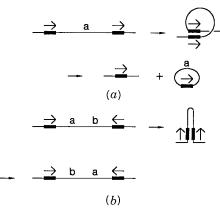
DISTRIBUTION OF REPEATS ALONG CHROMOSOMES |
509 |
Figure |
14.37 |
DNA rearrangements produced by recombination between interspersed repeats like |
|
the Alu |
sequence. |
(a) A direct repeat leads to a DNA deletion because the short fragment produced |
|
is unlikely to be |
retained or replicated. |
(b) An inverted repeat leads to an inversion in the DNA se- |
|
quence. |
|
|
|
The next most common human repeat is the L1 sequence. It sometimes called Kpn be- |
|
||||||
cause it has characteristic restriction sites for the enzyme Kpn I. The Kpn family is quite |
|
||||||
complex. The total sequence is about 6.4 kb in length. However, only 10% to 20% of the |
|
||||||
repeats are full length. Most others retain only the 3 |
|
|
-terminal kb of the L1. These 3 |
L1’s |
|||
occur at about a tenth the frequency of the Alu sequence. L1’s are |
more similar in pri- |
|
|||||
mates and rodents than Alu’s. |
Thus they must be used cautiously |
as |
species-specific |
|
|||
probes. L1 sequences are an example of the class of repeats called long interspersed re- |
|
||||||
peating sequences or LINES. Altogether the repeated sequences listed |
in |
Table |
14.3 add |
|
|||
up at most to 350 Mb of DNA. Centromeric satellite is estimated to account for another |
|
||||||
150 to 300 Mb of DNA. This material is tandemly repeating (Chapter 2). Thus at least |
|
||||||
100 Mb of the total estimated 750 Mb (25%) of repeated human DNA remains unac- |
|
||||||
counted for, and we may be missing as much half of all the repeated sequences. |
|
|
|
||||
Interspersed repeats appear to act as recombination hot spots. The sequence of most |
|
||||||
examples of Alu repeats is similar enough that recombination between pairs of such re- |
|
||||||
peats is sometimes seen as a cause of disease alleles. As shown in Figure 14.37, depend- |
|
||||||
ing on whether the repeats are head to head (tandem) or head to tail (inverted), the result |
|
||||||
of an intrachromosomal recombination event will be an inversion |
or |
a |
deletion. |
|
|||
Recombinations between repeats on different chromosomes will produce translocations. |
|
||||||
The low-density lipoprotein receptor is one of the genes where a deletion caused by inter- |
|
||||||
Alu recombination has been seen. In this case the result is to produce a disease allele for |
|
||||||
familial hypercholesterolemia. |
|
|
|
|
|
|
|
DISTRIBUTION OF |
REPEATS |
ALONG CHROMOSOMES |
|
|
|
|
|
In Chapter 2 we illustrated the fact that light bands and dark bands |
of human |
chromo- |
|
||||
somes had some very different general properties. A commonly accepted mechanism for |
|
|
|||||
the spread of interspersed repeats is that at least some of the copies of these sequences are |
|
||||||
mobile elements and |
can spread |
themselves or copies to other sites. This |
has |
definitely |
|
||