Добавил:

fench Опубликованный материал нарушает ваши авторские права? Сообщите нам.

Вуз:

Сумский государственный университет

Предмет:

Генетика

Файл:

Genomics- The Science and Technology Behind the Human Genome Project. Charles R. Cantor, Cassandra L / genomics11-15 / 15

.pdf

Скачиваний:

Добавлен:

17.08.2013

Размер:

499.07 Кб

Скачать

☆

1 / 51 2 3 4 5 > Следующая >>>

Genomics: The Science and Technology Behind the Human Genome Project.	Charles R. Cantor, Cassandra L. Smith
	Copyright © 1999 John Wiley & Sons, Inc.
	ISBNs: 0-471-59908-5 (Hardback); 0-471-22056-6 (Electronic)

15 Results and Implications of

Large-Scale DNA Sequencing

The accumulation of completed DNA sequences and the development and utilization of

software tools to analyze these sequences are changing almost daily. It is extremely frus-

trating to attempt an accurate portrait of this area in the kind of static snapshot allowed by

the written text. The authors know with certainty that much of this chapter will become

obsolete in the time interval it takes to progress from completed manuscript to published

textbook. This is truly an area where electronic rather than written communication must

predominate. Hence, while a few examples of original projections of human genome pro-

ject progress will be given, and a few

examples of actual progress will be

summarized,

the emphasis will be on principles that underlie the analysis of DNA sequence. Here it is

possible to be relatively brief, since a number of more complete and more advanced treat-

ments of sequence analysis already exist (Ribskaw and Devereaux, 1991; Waterman,

1995). The interested reader is also

encouraged to explore the databases and

software

tools available through the Internet (see the Appendix).

COSTING

THE

GENOME

PROJECT

When the lectures that formed the basis

of this book were given in the Fall

1992, there

were more than 37 Mb of ﬁnished DNA sequence from the six organisms chosen as the

major targets of the U.S. human genome project. The status in February 1997 of each of

these efforts is contrasted with the status ﬁve years earlier in Table 15.1. The clear im-

pression provided by Table 15.1 is that terriﬁc progress has been made on

E. coli, S. cere-

visiae,

and

C. elegans,

but we have a long way

to go

to complete the

DNA

sequence of

any higher organism. In addition to the six organisms listed in Table 15.1, a few other or-

ganisms like the plant model system

Arabidopsis thaliana

and the yeast

S. pombe

will

surely also be sequenced in the next decade along with a signiﬁcant number of additional

prokaryotic organisms.

Other attractive

targets for DNA sequencing would be

higher

plants with small genomes like rice, and higher animals

with

small

genomes

the

puffer ﬁsh. If methods are developed that allow efﬁcient differential sequencing (see

Chapter 12), methods that look just at sequence differences, some of the higher primates

become of considerable interest. Although these genomes are as complex as the human

genome, DNA sequences differences between them are only a few percent, and most of

these will lie in introns. Thus

a comparison between gorilla and

human

would

make it

very easy to locate small exons that might be missed by various computerized sequence

search methods.

different cast

provided

by the

ﬁgures in Table 15.2,

which

illustrate the average

rate of DNA sequencing per investigator up until 1990 since the ﬁrst 24 DNA bases were determined almost 30 years ago. The results in Table 15.2 show a steady rise in the rate of

526

			COSTING THE GENOME PROJECT				527
TABLE 15.1	Progress Towards Completion of the Human Genome Project

		Finished DNA Sequence (Mb)

Organism	Complete Genome	June 1992	February 1997	Comment

E. coli		4.6	3.4	4.6	Complete
S. cerevisiae		12.1	4.0	12.1	Complete
C. elegans		100	1.1	63.0	Cosmids		a
C. elegans		100	1.1	63.0	Cosmids
D. melanogaster		165	3.0	4.3	Large contigs only
M. musculus	3000		8.2	24.0	Total assuming
					2.5	redundant
H. sapiens	3000		18.0	31.0	In contigs,		10Kb
				116.0	Total assuming
					2.5	redundant

a Completion is expected at the end of 1998.

DNA sequencing. However, they understate this rise, since the data are derived from all DNA sequencing efforts. In practice, the majority of these sequencing efforts use simple, manual technology, and many are performed by individuals just learning DNA sequencing. The common availability and widespread use of automated DNA sequencing equip-

ment probably had little impact on the results in Table 15.2 because these advances are too recent. Despite this fact, the general impression, based on DNA sequences deposited into databases, is that the total accumulation of DNA sequences is increasing nearly exponentially with time, and this trend certainly has continued to the present.

A stated goal of the human genome project in the United States is to complete the DNA sequence of one haploid-equivalent human genome by the year 2005. Two immedi-

ate cautionary notes must be struck. First, the sequence is unlikely to really be completed

by then or perhaps by any time in the foreseeable future	because it is unlikely anyone
would want to, or could, sequence through millions of base	pairs of centromeric tandem

repeats, looking for occasional variations. Second, it may not be a single genome that is sequenced. A considerable amount of the material for DNA sequencing is likely to come

from cell lines containing particular human chromosomes.	In general, each line repre-
sents chromosomes from a different individual. Thus, to	whatever degree of completion

the ﬁrst human DNA sequence is obtained, it will surely be a mosaic of many individual genomes. In view of the nature of the task, and its importance to humanity, this outcome actually seems quite appropriate. It also answers, once and for all, the often-asked question “who will be sequenced in the human genome project?”

Setting the above complications aside, the chance of achieving the DNA sequencing goals of the human genome project depends principally on three variables: the amount of money available for the project as a whole, the percent of it used to support large-scale genomic sequencing, and the efﬁciency of that sequencing, namely the cost per base pair and how it evolves over the course of the project. In most current genomic DNA sequenc-

ing efforts, labor still appears to be the predominant cost, and all other considerations can be scaled to the number of individuals working. This is changing with the incorporation

of more and more highly automated methods; supplies and materials are becoming the dominant cost. However, since we cannot yet accurately estimate the impact of automation on sequencing costs, we will assume the continuation of dominant labor costs in order to make some projections.

528

T ABLE

15.2

Summary of Pr

ogr ess Made in DN

A Sequence

Analysis Between 1967 and 1990

Number of

Percent T ime

Nucleotides

Sequence

Nucleotides

In v estigators

for Sequencing

per Year ,per

Relati v e

Determined

Method(s)

T ime Period

Determined

In v olv ed

Steps

In v estigator

Speed

Cohesi

v e ends of

Partial incorporation;

1967–

1970

80 – 9 0

partial digestion

Cohesi

v e ends of 186p DN

Same as abo

v e

1971

–

1972

80 – 9 0

1 2

X174, f1

Mobility shift

1972

–

1973

140

40 – 50

2 8

X174

Plus-and-minus

1973

–

1977

5000

2 0 – 3 0

138

er 500 sequences

Dideoxy chain

1977

–

1982

66,000

350

20 – 3 0

380

termination

er 7000 sequences

Recombinant DN

1982

–

1986

9,000,000

3,500

15–25

640

160

M13 v

ectors,

etc.

er 40,000 sequences

Same as abo

v e ,

1986 –

1989

27,000,000

9,000

10–20

1000

250

automatic DN

A sequencer

er 23,000 sequences

Same as abo

v e

1989

–

1990

14,000,000

12,000

10–20

1160

290

Sour

ce:

Adapted from

W u (1993).

COSTING THE GENOME PROJECT

In most U.S. academic or pure research settings, an average person working in the lab-

oratory costs about $100,000 a year to support. This includes salary, fringe beneﬁts,

chemicals, supplies, and academic overhead such as administrative costs, light, heating,
and amortization of laboratory space. Let’s make the reasonably hard-nosed estimate that
the average genome sequencer will work 250 days per year. Dividing this into the yearly
cost results in a cost per working day	of $400. A reasonable estimate of state-of-the-art
DNA sequencing rates is about 10	4 raw base pairs per day per individual. Allowing for
20% waste, and dividing by a factor of 8 for the redundancy needed for shotgun strate-
gies, we can estimate that the sequencing rate for ﬁnished base pairs per day is 10
the daily cost is divided by the daily	output, the result is a cost per ﬁnished base pair of

$0.40. This is far lower than the current commercial charges for DNA sequencing services, which average several dollars per base, or the cost of more casual sequencing efforts which, based on the most recent rates shown in Table 15.2, weould be about $90 per

base. The cost per ﬁnished base of the		H. inﬂuenza		project recently completed was $0.48
in direct supplies and labor. This is equivalent to at least $1.00/bp when overhead and in-
strument depreciation costs are added.
Although the relatively low cost of current automated DNA sequencing is impressive,
compared to the cost of less systematic efforts, it falls far short of the economies that will
need to be achieved to complete the	human genome project	within	the allowable	budget
and time scale. The initial design of the U.S human genome project called for $3000 mil-
lion to be spent over 15 years. This would translate into a cost of $1 available per human
base pair if all one did was sequence. Such a plan would be ridiculous because it ignores
mapping, which provides the samples to be sequenced,		and it	does not allow for any
model organism work or technology development. The U.S. human			genome budget	in
1992 was $160 million per year. If we had ramped up to large-scale DNA sequencing im-
mediately, starting in October 1993, we would have had 12 years to complete the project.
A steady state sequencing rate model would have required sequencing at a rate of 250
million base pairs per year. At current best attainable costs this would require $100 mil-
lion per year to be spent on human genomic DNA sequencing. So			this way the project
could be completed, but to proceed with such a plan that anticipates no enhancements in
technology would be lunacy.
It is more sensible to scale up sequencing more gradually and to build in some as-
sumptions about improved efﬁciency. The caveat to this approach is that the slower the
scale up, the more efﬁcient the ﬁnal sequencing rates must become. Suppose that we arbi-
trarily limit the amount of funds	committed to human genomic DNA		sequencing to	the
$100 million annual costs required by the steady state model. Table 15.3 shows one set of
cost projections, developed in 1992 by Robert Robbins. At ﬁrst glance this may seem like
an extremely optimistic scenario, since it starts with average costs that are $1.50 per base
pair and requires only a factor of	ten decrease in unit cost over		a seven-year time period
to reach $0.15 per ﬁnished base pair by 2001. However, these are average costs, and at
these costs an average work force of 1000 individuals will			be needed for the last ﬁve
years of the project, just for human DNA sequencing. The bottom line is that the scenario
in Table 15.3 seems reasonable and achievable, but one hopes that some of the potential
improvements in DNA sequencing described in Chapters 11 and 12 will be realized and
will result in considerably faster	rates of sequence acquisition. From this point of view,
the scenario in Table 15.3 is actually quite pessimistic.
One way to view the cost effectiveness of the genome program is to ask how much ad-
ditional DNA sequencing will be accomplished beyond the		stated	goal of one	human

529

3 . When

530		RESULTS AND IMPLICATIONS OF LARGE-SCALE DNA SEQUENCING
	TABLE	15.3 One Model for DNA Sequencing Costs in the Human Genome Project

		Finished,	Annual		Genomic Sequence (Mb)			Percent of
		per-Base	Sequencing		Genomic Sequence (Mb)			Genome


	Year	Direct Cost	Budget ($millions)	Year		Cumulative	Completed

1995		$1.50	16		11		11	0.33
1996		$1.20	25		21		32	0.96
1997		$0.90	35		39		71	2.15
1998		$0.60	50		84		155	4.71
1999		$0.45	75		168		324	9.81
2000		$0.30	100		337		660	20.01
2001		$0.15	100		673		1334	40.42
2002		$0.15	100		673		2007	60.82
2003		$0.15	100		673		2681	81.23
2004		$0.15	100		673		3354	101.63

genome. If the development of new sequencing methods proceeds very well, it may be

possible to complete extensive portions of the mouse		genome, and perhaps even other
model organisms with large genomes, under the cost umbrella of funding for the human
sequence. This is not inappropriate, since the more		relevant model	organism sequence
data that we have available, the more powerful will be		our ability to	interpret		the human
DNA sequence.
Whether one adopts an optimistic or a pessimistic		scenario, the	inevitable		conclusion
is that by October 2005 or thereabouts, 3		10 9		base	pairs of human genomic DNA en-
coding for something like 100,000 human genes will be thrust upon the scientiﬁc commu-
nity. The challenge will be to ﬁnd any genes in the sequence that are not already repre-
sented as sequenced cDNAs, translate the DNA sequence into protein			sequence,		make
some preliminary guesses about the function of some of these proteins, and decide which
ones to study ﬁrst in more detail. The remainder of this chapter deals with these chal-
lenges. Because of the rapid advances in cDNA sequencing described earlier in Chapter
11, some of these challenges already confront us today.
FINDING	GENES
There are two very different basic approaches to ﬁnding the genes encoded for by a sam-
ple of	genomic DNA. The experimental approach is to use the DNA as		a probe (or a
source of probes or PCR primers) to screen available cDNA libraries. One can also use
available DNA materials to look directly at the mRNA population in different cell types.
This is most easily accomplished by Northern blots, as described in Chapter 13. None of
these approaches require that the DNA sequence be completed, and except for the synthe-
sis of PCR primers, none require any known DNA sequence. These pure experimental
methods	will succeed only if the mRNAs or cDNAs in question are present			in available

sources in sufﬁcient quantities to be detected above the inevitable background caused by nonspeciﬁc hybridization or PCR artifacts.

The second basic approach is the one that we will concentrate on here. It requires that the sequence of the DNA be known. Genes have characteristic sequence properties that

distinguish	them,	to	a considerable extent, from nongenic DNA or from random se-
quences. The	goal is	to	optimize the methods for making these discriminations. One triv-

FINDING GENES

531

ial procedure should always be tried to an newly revealed piece of genomic DNA. This is to compare its sequence with all known sequences. A near or exact match could immedi-

ately reveal genes or other	functional elements.		For	example,	large amounts	of partial
cDNA sequence information	are	accumulating	in	publicly	accessible	databases.

Frequently these cDNAs have already been characterized to some extent, such as their lo-

cation on	a human physical map or their	pattern of expression in various	tissues.	Finding
a genomic	match to such a cDNA fragment	clearly indicates the presence	of a gene	and

provides a jump start to further studies. The problem that arises is what if the match between a portion of the genomic DNA sequence and other molecules with known sequence

is not exact, or what if there is no signiﬁcant detectable match at all?

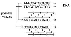
A number of basic features of genomic DNA sequence can be examined to look for the location of genes. The most straightforward of these is to search for open reading frames

(ORFs). This is illustrated in Figure 15.1. A given stretch of DNA sequence can potentially be translated into protein sequence in no less than six different ways. The triplet ge-

netic	code allows for three possible reading frames, and a priori either DNA strand (or
both) could be coding. Computer analysis is used to translate the DNA sequence into pro-
tein	in all six reading frames, and assemble these in order along the	DNA. The	issue is
then	to decide which represent actual segments of coding sequence and	which are	just
noise.
Almost all known patterns of mRNA transcription occur in one direction along a tem-
plate	DNA strand. Segments of the mRNA precursor are then removed	by splicing to

make the mature coding mRNA. The exceptions to this pattern are fairly rare in general, and the few organisms in which they are more frequent are fairly restricted. Some parasitic protozoa and some worms have extensive trans-splicing where a mRNA is composed

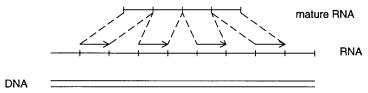
from units coded on different chromosomes. Editing of mRNAs, where DNA-templated bases are removed, individually, and bases not templated by DNA are added, individually, also appears to be a rare process concentrated in a few lower organisms. Thus it is almost always safe to assume that a true mRNA will be composed of one or more successive segments of DNA sequence organized, as shown schematically in Figure 15.2. The challenge

is to predict where the boundaries of the possible exons are, and where individual genes actually begin and end. This requires the simultaneous examination of aspects of the RNA sequence as well as aspects of the coded protein sequence.

True exons must have arisen by splicing. Thus the sequences near each splice site must resemble consensus splicing signal sequences. While these are not that well deﬁned, they

have	a	few speciﬁc characteristics that we can look for. True exon coding segments	can
have	no	stop codons, except at the very end of the gene. Thus the presence of	UAA,

UAG, or UGA can usually eliminate most possible reading frames fairly quickly. A true gene must begin with a start codon. This is usually AUG, although it can also be GUG,

Figure 15.1 Six possible reading frames from a single continuous stretch of DNA sequence shown earlier in Figure 1.13.

532 RESULTS AND IMPLICATIONS OF LARGE-SCALE DNA SEQUENCING

Figure 15.2	A message is read discontinuously from a DNA, but all of	the examples known		to
date are read from the same strand, in a strict linear order (except for the very specialized case of
transsplicing seen in some simple organisms).
UUG, or AUA. True start codons are context dependent. For example, a true AUG used
for starting translation must have nearby sequences that are used by the ribosome or pro-
tein synthesis	initiation factors (proteins) to bind the message and	initiate	translation.
These residues usually lie just upstream from the AUG, but they can also extend a bit
downstream.
The key factor in determining the correct points for the initiation of translation is that
the context of starting AUGs is very species dependent. Thus, since the		species of	origin
of a DNA will almost always be known in advance, a great deal of information can be
brought to bear to recognize a true start. For example, in			E. coli,		a given mRNA can have
multiple starting AUGs within a message because		E.	coli	commonly makes and uses
polycistronic messages. In eukaryotes, messages are usually monocistronic. Most fre-
quently it is the ﬁrst AUG in the message that signals the start of translation. This means
that information about transcription starting signals or splicing signals		must be	used to
help locate the true starting points for translation of eukaryotic DNA sequences.
A true mRNA must also have a transcription stop. This is relatively easy to ﬁnd in
prokaryotes. However, we still know very little about transcription termination in eukary-
otes. Fortunately, most eukaryotic mRNAs are cleaved, and a polyA tail is added. The
consensus sequence for this process is AATAAA. This is distinct, but it is very short, and
such a sequence can easily occur by random ﬂuctuations in A				T-rich mammalian DNA.
This polyA addition signal is an example of a fairly general problem in sequence analy-
sis. Many control sequences are quite short; they often work in concert with other control
elements, and we do not yet know how to recognize the overall pattern.

MORE ROBUST METHODS FOR FINDING GENES BY

DNA SEQUENCE ANALYSIS

If the methods just described represented all of the available information, the task of ﬁnding previously unknown genes by genomic DNA sequence analysis alone would be all

but hopeless. Fortunately a great deal of additional information is available. Here we will describe some of the additional characteristics that distinguish between coding and noncoding DNA sequences. The real challenge is to ﬁgure out the optimal way to combine all

of this additional knowledge into the most powerful prediction scheme. A simple place to start is to consider the expected frequency of each of the 20 amino acids. Some, like tryptophan, are usually very rare in proteins; others are much more common. A true coding

sequence will, on average, contain relatively few rare amino acids. Similarly the overall

average amino acid	compositions of	proteins	vary, but they	usually lie within certain
bounds. A potential	coding sequence	that led	to a very extreme	amino acid composition

MORE ROBUST METHODS FOR FINDING GENES BY DNA SEQUENCE ANALYSIS											533
would usually be rejected if an alternative model for the translation of this segment of the
DNA led to a much more normal amino acid composition. Note that the argument we are
using is one of plausibility, not certainty. Statistical weights have to be attached to such
arguments to make them useful. The same sort of considerations will apply to all of the
other measures of coding sequence that follow.
The genetic code is degenerate. All amino acids except methionine and tryptophan can
be speciﬁed by multiple DNA triplet codons. Some amino acids have as many as six pos-
sible codons. The relative frequency at which these synonymous codons are used varies
widely. In general, codon usage is very uneven and is very species speciﬁc. Even different
classes of genes within a given species have characteristic usage patterns. For example in
highly expressed	E. coli	genes the relative frequencies				of arginine codon use				per	1000
amino acids are
		AGG		0.2		CGG			0.3
		AGA	0.0			CGA			42.1
		CGA		0.2		CGC			13.9
These nonrandom values have a signiﬁcant effect on the selection of real open reading
frames.
Some very interesting biological phenomena underlie the skewed statistics of codon
usage. To some extent, the distribution of highly used codons must match the distribution
of tRNAs capable of responding to these codons; otherwise, protein synthesis could not
proceed efﬁciently. However, many other factors				participate.	Codon	choice	affects		the
DNA sequence in all reading frames; thus the choice of a particular codon may be medi-
ated, indirectly, by the desire to avoid or promote a particular sequence in one of the other
reading frames. For example, particular codon use near the starting point of protein syn-
thesis can have the effect of strengthening or weakening the ribosome binding site of the
mRNA. Rare codons usually correspond to rare tRNAs. This in turn will result in a pause
in protein synthesis, while the ribosome-mRNA complex waits for such a tRNA to									ap-
pear. This sort of pausing appears to be built into the sequence of many messages, since
pausing at speciﬁc places, like domain boundaries, will assist the newly synthesized pep-
tide chain to fold into its proper three-dimensional conﬁguration.
Codon usage can also serve to encourage or avoid certain patterns						of DNA	sequence.
For example, DNA sequences with successive A’s spaced one helical repeat apart							tend to
be bent. This may be desirable in some regions and not in others. Inadvertent promoter-
like sequences in the middle of actively transcribed genes are					probably best		avoided, as
are accidental transcription terminators. The			ﬂexibility of the genetic code					that	results
from its degeneracy allows organisms to synthesize whatever proteins they need, while
avoiding these potential complications. For example, a continuous stretch of							T’s forms
part of one of the transcription termination signals in								E. coli.		The resulting triplet, UUU,
which codes for phenylalanine occurs only a third as often as the synonymous								codon,
UUC. Another example is seen with codons that signal termination of						translation. UAA
and UAG are two commonly used termination signals. The complements of these signals
are UUA and CUA. These are both codons			for	leucine; however,		CUA	is	the	rarest
leucine codon, and UUA is also rarely used.
There are many	additional constraints on		coding sequences		beyond	the statistics of

codon usage. In real protein sequences there are some fairly strong patterns in the occurrence of adjacent amino acids. For example, in a beta sheet structure, adjacent amino acid

534 RESULTS AND IMPLICATIONS OF LARGE-SCALE DNA SEQUENCING

side chains will point in opposite directions. Where the beta sheet forms part of the structural core of a protein domain, usually one side will be hydrophobic and face in toward the center of the protein, while the other side will be hydrophilic and face out toward the solvent. Thus codons that specify nonpolar residues will tend to alternate to some extent with codons that specify charged or polar residues. Alpha helices will have different patterns of alternation between polar and nonpolar residues because they have 3.4 residues

per	turn. In	many protein structures one face of many	of the alpha helices will be polar
and	one face	will be nonpolar. These are not absolute	rules; however, alpha helices and

beta sheets are the predominant secondary structural motifs in proteins, and as such, they cast a strong statistical shadow over the sorts of codon patterns likely to be represented in a sequence that actually codes for a bona ﬁde mRNA.

Quite a few other characteristics of known proteins seem to be general enough to affect the pattern of bases in coding DNA. Certain dipeptides like trp-trp and pro-pro are usually very rare; an exception occurs in collagenlike sequences, but then the pattern pro- pro-gly will be overwhelmingly dominant. Repeats and simple sequences tend to be rare inside of coding regions. Thus Alu sequences are unlikely to be seen within true coding

regions; blocks like		AAATTTCCCGGG		. .	. are	also conspicuously rare. VNTRs are
also usually absent in coding sequences, although there are some notable exceptions like
the	androgen receptor	which	contains three simple sequence	repeats.	Such	exceptions
may	have important biological consequences, but we do not understand them yet. All of
these statistically nonrandom			aspects of protein sequence imply	that we	ought	to be able

to construct some rather elaborate and sophisticated algorithms for predicting ORFs and splice junctions. Seven of these that were used in the ﬁrst successful algorithms for ﬁnding genes are described below.

Frame Bias

In a true open reading frame (ORF), the sequence is parsed so that every fourth base must

be the beginning	of	a codon. If we represent a reading frame as (		)	n , in a true reading
frame the bases	in	each position should tend to be those consistent		with the	preferred
codon usage in the particular species observed. The other possible			reading frames should
tend to be those with		poor codon usage. In this way the possibility	of accidentally reading
a message in the wrong frame will be minimized.

Fickett Algorithm

This is an amalgam of several different tests. Some of these examine the 3-periodicity of each base versus the known properties of coding DNA. The 3-periodicity is the tendency

for the same base to recur in the 1st, 4th, 7th		, . .	. positions. Other tests look at the over-
all base composition of the sequence.
Fractal Dimension
Some dinucleotides are rare, while	others are common. The fractal dimension		measures
the extent to which common codons	are clustered with	other common ones,	and rare

codons are clustered with other rare ones. Clustering of similar codon classes is characterized by a low fractal dimension, while alternation will lead to a high fractal dimension. It turns out that exons have low fractal dimensions, while introns have high fractal dimen-

NEURAL NET ANALYSIS OF DNA	SEQUENCES	535
sions. Thus this test combines some features of codon usage, common dipeptide se-
quences, and simple sequence rejection.
Coding Six-Tuple Word Preferences
A six-tuple is just a set of six continuous DNA bases. There are 4	6possible six-tuples	in
DNA. Since we have tens of millions of base pairs of DNA to examine for some species,
we can make reasonable projections of the likely occurrence of each of these six-tuples in
coding sequences versus noncoding sequences. An appropriately weighted sum of these
predictions will allow an estimate of the chances that a given segment is coding.

Coding Six-Tuple In-Frame Preferences

In this algorithm one computes the relative occurrence of preferred six-tuples in each possible reading frame. For true coding sequence, the real reading frame should show an excellent pattern of preferences, while in the other possible reading frames, when actual coding sequences have been examined, the six-tuple preferences appear to be fairly poor. This presumably aids in the selection and maintenance of the correct frame by the ribosome. This particular test turns out to be a very powerful one.

Word Commonality

This test is also based on the statistics of occurrences of six-tuples. Introns tend to use very common six-tuples; exons tend to use rare six-tuples. Note that here we are talking about the overall frequency of occurrence of six-tuples and not their relative frequency in coding or noncoding regions.

Repetitive Six-Tuple Word Preferences

This test looks speciﬁcally at the six-tuples that are common in the major classes of repeating DNA sequences. These six-tuples will also tend to be rare in true coding sequences.

The large list of tests just outlined raises an obvious dilemma: which one should be picked for best results? However, this is not an efﬁcient way to approach such a problem. Instead, what one aims to do is ﬁnd the optimal way to integrate the results of all of these tests to maximize the discrimination between coding and noncoding DNA. One must be

prepared for the fact that the optimum measure will be species dependent; in addition it may well be dependent on the context of the particular sequence actually being examined.

In other words, no simple generally applicable rule for combining the test results into a single score representing coding probability is likely to work. Instead, a much more sophisticated approach is needed. One such approach, which has been very successful, uses the methodology of artiﬁcial intelligence algorithms.

NEURAL NET ANALYSIS OF DNA SEQUENCES

A neural net is one form of artiﬁcial intelligence. It is so named because, with neural net algorithms, one attempts to mimic the behavioral characteristics of networks of neurons.

1 / 51 2 3 4 5 > Следующая >>>

Соседние файлы в папке genomics11-15

#
17.08.2013277.66 Кб4711.pdf
#
17.08.2013510.17 Кб4612.pdf
#
17.08.2013311.59 Кб4613.pdf
#
17.08.2013577.75 Кб4514.pdf
#
17.08.2013499.07 Кб4715.pdf
#
17.08.201326.85 Кб46appendix databases.pdf