

556 RESULTS AND IMPLICATIONS OF LARGE-SCALE DNA SEQUENCING
Figure 15.23 Results of two actual comparisons between polyoma and SV40 viral DNA sequences, computed as described for the hypothetical example in Figure 15.22. Dots show DNA
windows with more than 55% identity within a window (top) or more than 66% (bottom). Provided by Rhonda Harrison.

|
|
|
|
DYNAMIC |
PROGRAMMING |
557 |
|
strong homology show up as a series of dots along a |
diagonal in |
these plots. |
One can |
|
|
|
|
piece together the set of diagonals found to construct a model for a global alignment in- |
|
|
|
||||
volving all the residues. However, it is not easy to show if a particular global alignment |
|
|
|||||
reached in this manner is the best one possible. |
|
|
|
|
|
|
|
DYNAMIC |
PROGRAMMING |
|
|
|
|
|
|
Dynamic programming is a method that improves on the dot matrix approach just de- |
|
|
|
||||
scribed because it has the power, in principle, to find an optimal sequence alignment. The |
|
|
|
||||
method is computationally intensive, but not beyond the capabilities of current supercom- |
|
|
|
||||
puters or specialized computer architectures or hardware designed to perform such tasks |
|
|
|
||||
rapidly and efficiently (Shpaer et al., 1996). The basic notion in dynamic programming is |
|
|
|||||
illustrated in Figure 15.24. Here an early stage in the comparison of two |
sequences |
is |
|
|
|||
shown. Gaps are allowed, but a statistical penalty (a loss in total similarity score) is paid |
|
||||||
each time a gap is initiated. (In more complex schemes the penalty can depend on the size |
|
|
|
||||
of the gap.) We already discussed the fiercely difficult combinatorial problem that results |
|
|
|
||||
if one tries out all possible gaps. However, with dynamic programming, in the example |
|
|
|
||||
shown in Figure 15.24, one argues that the best alignment achievable at point |
|
|
|
n (n is the |
|||
total number of residues plus gaps that have been inserted into |
either of the |
sequences |
|
|
|
||
since start of the comparison) must contain the best |
alignment at |
point |
plus |
the |
n |
1, |
|
best scoring of the following three possibilities: |
|
|
|
|
|
|
|
1. |
Align the two residues at position |
n . |
|
|
|
|
|
2.Gap the top sequence.
3.Gap the bottom sequence.
The argument behind this approach is not totally rigorous. There is no reason why the optimal alignment of two sequences should be co-linear. DNA rearrangements can change the order of exons, invert short exons, or otherwise scramble the linear order of genetic information. Dynamic programming, as conventionally used, can only find the optimal co-linear alignment. However, one can circumvent this problem, in principle, by attempting the alignments starting at selected internal positions in both possible orientations, and determining if this alters the best match obtained.
Figure 15.24 Basic methodology used in comparison of two sequences by dynamic programming.

558 |
RESULTS AND IMPLICATIONS OF LARGE-SCALE DNA SEQUENCING |
|
|
|
Sequence alignment by dynamic programming is conveniently viewed by a plot |
as |
|
shown in Figure 15.25. The coordinates of the plot are the two sequences, just |
as |
in the |
|
dot matrix blot discussed earlier. However, what is plotted at each position is not a score |
|||
from |
the comparison of two sequence windows; instead, it is a cumulative score |
for |
a |
path through the two sequences that represents a particular comparison. In the simple ex- |
|
||
ample in Figure 15.25, the scoring is just for identities. In a real case, the elements of a |
|||
scoring matrix would be used. From the example in Figure 15.25 |
|
a it can be seen that a |
|
particular alignment is just a path of arrows between adjacent residues. The three possible steps listed above at a given point in the comparison just correspond to:
1.Advancing along a diagonal
2.Advancing horizontally
3.Advancing vertically
In dynamic programming one must consider all possible paths through the matrix. A particular comparison is a continuous set of arrows. The best comparisons will give the highest scores. Usually there are multiple paths that give equal, optimal alignments. These can be found by starting with the point in the plot with the highest score and tracing back toward the beginning of the sequence comparison to find the various routes that can lead to
this final point (Fig. 15.25 |
b ). |
Rigorous dynamic programming is |
a very computationally intensive process because |
there are so many possible paths to be tested. Remember that for each new protein sequence, one wishes to test alignments with all previously known sequences. This is a very
Figure 15.25 |
A simple example of dynamic programming. |
(a) Matrix |
used to describe the scores |
of various alignments |
between two sequences. Note that successive horizontal and |
vertical moves |
|
are forbidden, since this introduces a gap on both strands which is equivalent to a diagonal move— |
|
||
not a gap at all. In |
each cell only the route with the highest possible score |
is shown. In practice, |
|
each cell can be approached in three different ways—diagonally, horizontally, |
and vertically. |
(b) |
|
The trace back through the matrix from the highest scoring configuration to find all paths (align- |
|
||
ments) consistant with that final configuration. Only the path with the highest score is kept. |
|
||

|
|
|
|
|
|
|
|
|
DYNAMIC PROGRAMMING |
559 |
|
large number of dynamic |
programming comparisons. A number of different |
procedures |
|
|
|
|
|||||
can be used to speed this up. Some pay the price of a loss of rigor, so no guarantee exists |
|
||||||||||
that the very best alignment will be found. |
|
|
|
|
|
|
|
|
|||
A very popular program for global database searching has been developed by David |
|
|
|||||||||
Lipman and his coworkers. This is called FASTA for nucleic acid comparisons, FASTP, |
|
||||||||||
for protein (or translated ORF) comparisons. The test protein |
is |
|
broken |
into |
k-tuple |
||||||
words. These are searched through the entire database, in looking for exact matches and |
|
||||||||||
scoring them. Some of these best scoring comparisons will form diagonal regions of dot |
|
|
|||||||||
plots with a high density of exact matches. The 10 best of these regions are rescored with |
|
||||||||||
a more accurate comparison matrix. They are trimmed to remove residues not contribut- |
|
|
|
||||||||
ing to the good score. Then nearby regions are joined, using gap penalties for the in- |
|
||||||||||
evitable gaps required in this process. The resulting sets of comparisons are examined to |
|
||||||||||
find those with the best, provisional fits. Then each of these is examined by dynamic pro- |
|
||||||||||
gramming within a relatively narrow band of 32 residues around the sites of each of the |
|
||||||||||
provisional matches. Even faster algorithms exist, like Lipman’s |
BLAST |
which |
looks |
|
|||||||
only at short exact fits |
but makes a rigorous statistical assessment of their |
significance. |
|
||||||||
This is used to winnow down the vast array of possible comparisons before more rigor- |
|
|
|||||||||
ous, and time-consuming, methods are employed. |
|
|
|
|
|
|
|
|
|||
A key point in favor of the dynamic programming method is that for each comparison |
|
|
|
||||||||
cell, as shown in Figure 15.26, one only needs to consider three |
immediate |
precursors. |
|
||||||||
This allows the computation to be broken into a set of steps that can be computed in par- |
|
||||||||||
allel. The comparison can proceed down the diagonal of the plot in waves, with each cell |
|
|
|||||||||
computed |
independently |
of |
what is happening in the other cells along |
that |
diagonal |
|
|||||
(Fig. 15.26). Thus parallel processing computers are well adapted to the dynamic |
|
||||||||||
programming method. The result is an enormous increase in our power |
to |
|
do |
global |
|
|
|||||
sequence comparisons. Using a parallel architecture, it is possible, |
|
with |
the |
existing |
|
||||||
protein |
database, to do |
a complete inversion. That is, all sequences |
are |
compared |
|
with |
|
||||
all sequences by dynamic |
programming. The resulting set of scores allows the |
database |
|
|
|||||||
to be factored into sequence families, and new, unsuspected sets of |
families |
have |
been |
|
|||||||
found in this way. As an |
alternative to parallel processing, specialized |
computer |
chips |
|
|||||||
have been designed and built that perform dynamic programming sequences |
|
compar- |
|
|
|
||||||
isons, but they do this very quickly because each sequence needs to be passed through the |
|
||||||||||
chip only once. |
|
|
|
|
|
|
|
|
|
|
|
Figure 15.26 Parallel processing in dynamic programming. Only three preceding cells are needed to compute the contents of each new cell. Computation can be carried out on all cells of the next diagonal, simultaneously.
560 RESULTS AND IMPLICATIONS OF LARGE-SCALE DNA SEQUENCING
GAINING ADDITIONAL POWER IN SEQUENCE COMPARISONS
With increases in available computation power occurring almost continuously, it is undeniably tempting to carry sequence comparisons even further to make them more sensitive.
The goal is to identify, as related, two or more sequences that lie at the edge of statistical certainty by ordinary methods. There are at least two different ways to attempt to do this.
One can try to introduce information |
about possible protein three-dimensional structure |
|
for the reasons described earlier in |
this chapter. Alternatively, one can attempt to |
align |
more than two sequences at a time. |
|
|
If two proteins are compared at the amino acid sequence level, but one of these |
pro- |
|
teins is of known three-dimensional structure, the sensitivity of the scoring used can be improved considerably, as we hinted earlier. One can postulate that if the two proteins are truly related, they should have a similar three-dimensional structure. In the interior of this structure, spatial constraints are very important. Insertions and deletions there will be very disruptive, and thus they should be assigned very costly comparison weights. The ef-
fects will be much less serious on the protein surface. Changes in any charged residues on the interior of the protein are also likely to be very costly. Interchanges among internal hydrophobic residues are likely to be tolerated, especially if there are compensating increases in size at some points and decreases in size elsewhere. Changes that convert internal hydrophobic residues to charged residues will be devastating. A small number of external hydrophobic residues may not be too serious. Changes in sequence that seriously destabilize prominent helices and beta sheets are obviously also costly.
A systematic approach to such structure-based sequence comparisons is called threading. Here the sequence to be tested is pulled through the structure of the comparison sequence. At each stage some structure variations are allowed to see if the new sequence is compatible in this alignment with the known structure. The effectiveness of threading procedures in improving homolog matching and structure prediction is still somewhat
controversial. However, in principle, this appears to be |
a very powerful method as more |
|
|||
and more proteins with known three-dimensional structures become available. |
|
|
|
||
As originally implemented by Christian Sander, by |
attempting |
to fit |
proteins |
of |
un- |
known structure to the various known protein structures |
as just |
described |
above, |
one |
|
gained 5% to 10% in the fraction of the database that showed significant protein similarity matches. Clearly this approach will improve significantly as the body of known pro-
tein structures increase in size. Another aspect of the protein structure fitting problem deserves mention here. As more and more proteins with known three-dimensional structure
become available, it is of interest to ask whether any pairs of proteins have similar threedimensional structure, outside of any considerations about whether they have similar amino acid sequences. Sander has constructed algorithms that can look for similar structures, essentially by comparing plots of sets of residues that approach each other to within less than some critical distance. Such comparisons have revealed cases where two very similar three-dimensional structures had not been recognized before because they were being viewed from different angles that obscured visual recognition of their similarity. In the future we must anticipate that the number of structures will be so great that no visual comparison will suffice, unless there is first a detailed way to catalog or group the structures into potentially similar objects.
The second approach to enhanced protein sequence comparison is multiple alignments. This allows weak homology to be recognized if a family of related proteins is assembled. Suppose, for example, that one saw a sequence pattern like
|
|
DOMAINS |
AND MOTIFS |
561 |
TABLE 15.6 |
One-Letter Code for Amino Acids |
|
|
|
|
|
|
|
|
One-Letter |
Three-Letter |
Amino Acid |
|
|
Code |
Code |
Name |
Mnemonic |
|
|
|
|
|
|
A |
ala |
alanine |
a lanine |
|
C |
cys |
cysteine |
c ysteine |
|
D |
asp |
aspartate |
aspar |
d ate |
E |
glu |
glutamate |
glutamat |
e |
F |
phe |
phenylalanine |
fenylalanine |
|
G |
gly |
glycine |
g lycine |
|
H |
his |
histidine |
h istidine |
|
I |
ice |
isoleucine |
isoleucine |
|
K |
lys |
lysine |
knear l |
|
L |
leu |
leucine |
leucine |
|
M |
met |
methionine |
m |
ethionine |
N |
asn |
asparagine |
asparagi |
n e |
P |
pro |
proline |
p roline |
|
Q |
gln |
glutamine |
“cute” amine |
|
S |
ser |
serine |
s erine |
|
T |
thr |
threonine |
threonine |
|
V |
val |
valine |
v aline |
|
W |
trp |
tryptophan |
t |
w yptophan |
Y |
tyr |
tyrosine |
t |
y rosine |
|
|
|
|
|
—P—AHQ—L—
in two proteins. Here we use the convenient one letter code for amino acids summarized
in Table 15.6. Such a pattern would be far too small to be scored as statistically significant. However, seeing this pattern in many proteins would make the case for all of them
much stronger. Currently most multiple alignments are done by making separate pairwise comparisons among the proteins of interest. The extreme version of this is the database inversion described previously. The use of pairwise comparisons throws away a considerable amount of useful information. However, it saves massive amounts of computer time. The alternative, for rigorous algorithms, would be dynamic programming in multiple di-
mensions. This is not a task to be approached by the faint of heart (or short of budget) with current computer speeds. Future computer capabilities could totally change this.
DOMAINS AND MOTIFS
From an examination of the proteins of known three-dimensional structure, we know that much of these structures can be broken down into smaller elements. These are domains,
independently folded units, motifs, and structural elements or patterns that describe the basic folding of a section of polypeptide chain, to form either a structural backbone or framework for a domain or a binding site for a ligand. Examples are various types of barrels formed by multiple-stranded beta sheets, zinc fingers and helix-turn-helix motifs, both of which are nucleic acid binding elements, Rossman folds and other ways of binding common small molecules like NAD and ATP, serine esterase active sites, transmem-

562 RESULTS AND IMPLICATIONS OF LARGE-SCALE DNA SEQUENCING
brane helices, kringles, and calcium binding sites. A few of these motifs are illustrated schematically in Figure 15.27. The motifs are not exact, but many can be recognized at the level of the amino acid sequence by conserved patterns of particular residues like cysteines or hydrophobic side chains.
Several aspects of the existence of protein motifs should aid our ability to analyze the function of newly discovered sequences once we understand these motifs better. First, there may well be just a finite number of different protein motifs, perhaps just several hundred, and eventually we will learn to recognize them all. Our current catalog of motifs derives from a rather biased set of protein structures. The current protein data base is composed mostly of materials that are stable, easy to crystallize, and obtainable in large quantities. Eventually the list should broaden considerably.
Each protein motif has a conserved three-dimensional structure, and so once we suspect a new protein of possessing a particular motif, we can use that structure for enhanced sequence comparisons as described above. If, as now seems likely, proteins are mostly composed of fixed motifs, any new sequence can be dissected into its motifs, and these can be analyzed one at a time. This will greatly simplify the process of categorizing new structures. However, the key aspect of motifs that makes them an attractive path from sequences to biological understanding is that motifs are not just structural elements, they
(a ) |
|
(b ) |
(c ) |
(d ) |
Figure 15.27 |
Some |
of the striking structural and functional motifs found in protein structures. ( |
a ) |
|
Helix-turn-helix. ( |
b |
) Zinc finger. ( c ) Beta barrel. ( |
d ) Transmembrane helical domain. |
|
INTERPRETING NONCODING SEQUENCE |
563 |
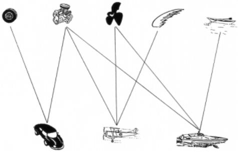
Figure 15.28 An example of how motifs (found in transportation vehicles) can be used to infer or relate the structures of composites of motifs.
are functional elements. There must be a relatively finite set of rules that determines what combinations of motifs can live together within a protein domain. Once we know these rules, our ability to make intelligent guesses about function from structural information alone should improve markedly.
One way to view motifs is to consider them as words in the language of protein function. What we do not yet know, in addition to many of the words in our dictionary, is the grammar that combines them. Another way to view protein motifs is the far-fetched, but perhaps still useful, analogy shown in Figure 15.28. This portrays various transportation vehicles and some of the structure-function motifs that are contained in them. If we knew
the function of the individual motifs, and had some idea about how they could be combined, we might be able to infer the likely function of a new combination of motifs, even though we had never seen it before; for example, we should certainly be able to make a good de novo guess about the function of a seaplane.
INTERPRETING NONCODING SEQUENCE
Most of the genome is noncoding, and arguments about whether this is garbage, junk, or potential oil fields have been presented before. The parts of the noncoding region that we are most anxious to be able to interpret are the control sequences which determine when, where, and how much of a given gene product will be made. Our current ability to do this is minimal, and it is confounded by the fact that most of the functional control elements appear to be very short stretches of DNA sequence. These sequences are not translated, so
we have only the four bases to use for comparisons or analyses. This leads to a situation with very poor signal to noise. In eukaryotes, control elements appeared to be used in

564 RESULTS AND IMPLICATIONS OF LARGE-SCALE DNA SEQUENCING
complex combinations like the example shown schematically in Figure 15.29. To analyze of stretch of DNA sequence for all possible combinations of small elements that might be
able to come together in such a complex seems intractable by current methods. Perhaps,
after we have learned much more about |
the properties of some of these control regions, |
|||
we will be able to do a better job. The true magnitude of this problem, currently, is well |
||||
illustrated by the globin gene family where one key, short control element required for |
||||
correct tissue-specific gene expression was found (experimentally, and after much effort) |
||||
to be located more than 20-kb upstream from the start of transription. Thus finding con- |
||||
trol elements is definitely not like shooting fish in a barrel. |
||||
DIVERSITY |
OF |
DNA |
SEQUENCES |
|
We cannot be interested in just the DNA sequence of a single individual. All of the intel- |
||||
lectual interest |
in studying both inherited human diseases and normal human variations |
|||
will come from comparisons among the |
sequences of different individuals. This is al- |
|||
ready done when searching for disease genes. Its ultimate manifestations may be the kind |
||||
of large-scale diagnostic DNA sequencing postulated in Chapter 13. |
||||
How different are two humans? From recent DNA sequencing projects (hopefully on |
||||
representative regions, but there is |
no way we can be sure of this) differences between |
|||
any two homologous chromosomes occur at a frequency of about 1 in 500. Scaled to the |
||||
entire human |
genome, |
this is 6 |
10 6 differences between any two chromosomes of a |
|
single individual, and potentially four times this number when two individuals are compared, since each homolog in one genome must be compared with each pair of homologs
in the other. To simply make a catalog of all of the differences for any potential individual against an arbitrary reference haploid genome would require 12
Figure 15.29 |
Structure of |
a typical upstream regulatory region for |
a |
eukaryotic gene. |
(a) |
Transcription factor-binding sequences. |
(b) Linear complex |
with |
transcription factors. |
(c) Three- |
|
dimensional structure of transcription factor-DNA complex that generates a binding site for RNA |
|
||||
polymerase. |
|
|
|
|
|
|
|
|
SOURCES AND |
ADDITIONAL READINGS |
565 |
||
The current population of the earth is around 5 |
|
|
10 9 individuals. Thus, |
to record all |
|||
of current human diversity would |
require a database with |
12 |
|
|
10 6 5 10 9 6 |
||
10 16 entries. By today’s mass storage standards, this is a large |
database. The entire se- |
|
|||||
quence of one human haploid genome could be stored on a single CD rom. On this scale, |
|
||||||
storage of the catalog of human diversity would require 2 |
|
|
|
10 7 CD roms, hardly some- |
|||
thing one could transport conveniently. However, computer mass storage has been im- |
|
||||||
proving at least by 10 |
4 per decade, and there |
is no sign that this rate of increase is slack- |
|
||||
ening. As a result, by the time we have the tools to acquire the complete record of human |
|
||||||
diversity, some 15 to 20 years from now, we should be able to store it on whatever is the |
|
||||||
equivalent, then, of a few CD roms. Genome analysis is unlikely to be limited now, or in |
|
||||||
the future, by computer power. |
|
|
|
|
|
|
|
Why would anyone want to view all of human diversity? There are two basic features |
|
||||||
that make this information compellingly interesting. First |
is the complexity of a number |
|
|||||
of interesting phenotypes that are undoubtedly controlled |
by many genes. Included are |
|
|||||
such items as personality, affect, and facial features. Given the limited ability for human |
|
||||||
experimentation, if we want to dissect some of the genetic |
contributions |
to |
these aspects |
|
|||
of our human characteristics, we will have to be able to compare DNA sequences with a |
|
||||||
complex set of observations. The more sequence we have, and the broader the range of |
|
||||||
individuals represented, the more likely it seems we should be able to make progress on |
|
||||||
problems that today seem totally intractable. |
|
|
|
|
|
||
The second motivation for studying the vast expanse of human diversity is a burgeon- |
|
||||||
ing field called molecular anthropology. A considerable amount of human prehistory has |
|
||||||
left its |
traces in our DNA. Within contemporary sequences should be a |
record of |
who |
|
|||
mated with whom as far back as our species goes. Such a record, if we could untangle it, |
|
||||||
would provide information about our past that probably cannot be reconstructed so easily |
|
||||||
and accurately in any other way. Included will be information about mass migrations, like |
|
||||||
the colonization of the new world, population expansions in prehistory, catastrophes, like |
|
||||||
plagues, or major climatic fluctuations. A tool that is useful for such studies is called prin- |
|
||||||
ciple component analysis. It looks at DNA or protein sequence variations |
across |
geo- |
|
||||
graphic regions and attempts to factor out particular variants with localized geographic |
|
||||||
distribution, or with gradients of geographic distribution. |
|
|
|
|
|
||
Many of the results obtained thus far in molecular anthropology are controversial and |
|
||||||
open to alternative explanations. As the body of sequence data that can be fed into such |
|
||||||
analyses grows, the robustness of the method and acceptance of its results will probably |
|
||||||
increase. Junk DNA may be especially useful for these kinds of analyses. It is much more |
|
||||||
variable |
between individuals than |
coding sequences, and thus the amount of |
information |
|
|||
it contains about human prehistory should be all that greater. One final, intriguing source |
|
||||||
of information is available from occasional DNA samples found still intact in mummies, |
|
||||||
human remains trapped in ice, or other environments that preserve DNA molecules. Such |
|
||||||
information will provide benchmarks by which to test the |
extrapolations |
that otherwise |
|
||||
have to be made from contemporary DNA samples. |
|
|
|
|
|
||
SOURCES |
AND ADDITIONAL READINGS |
|
|
|
|
|
|
Adams, M. D., Kelley, J. M., Gocayne, J. D., Dubnick, M., Polymeropoulos, M. H., et al. 1991. |
|
Complementary DNA sequencing: Expressed sequence tags and human genome project. |
Science |
252: 1651–1656. |
|