

Broadband Packet Switching Technologies
.pdf248 THE TANDEM-CROSSPOINT SWITCH
the same input buffer are destined to the same output port is 1rN. When N is small, Psuc is large. As a result, the later cell in the input buffer is likely to be blocked ŽNACK is received. because the first cell is still being handled in the tandem crosspoint. On the other hand, if N is large, Psuc is small, i.e., the blocking probability is small. The maximum throughput approaches 1.0 with
N ™ , because of Psuc ™0. In the double-speedup switch, the maximum throughput decreases to a certain value with increasing N, as is true for the
input buffering switch. Thus, the maximum throughput of the TDXP switch is higher than that of the double-speedup switch when N is large.
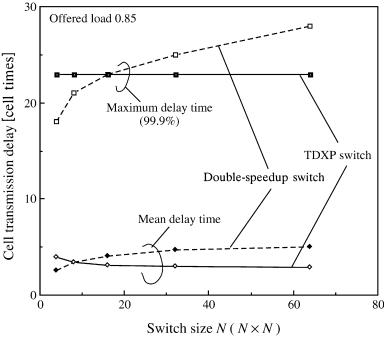
The cell transmission delay of the TDXP switch is compared with that of the double-speedup switch with N s 32. The maximum delay, defined as the 99.9% value, and the average delay are shown in Figure 9.6. The maximum and average delay of the TDXP switch are almost the same as those of the double-speedup switch with small ŽF 0.85.. However, when the offered load is larger than 0.85, the maximum and average delay values of the double-speedup switch increase strongly, because the limitation of the maximum throughput is smaller than that of the TDXP switch. In the TDXP switch, although the internal speed is the same as that of the input and output lines and a cell is buffered in a tandem crosspoint before it is
Fig. 9.6 Delay performance.
PERFORMANCE OF TDXP SWITCH |
249 |
Fig. 9.7 Delay performance vs. switch size. Ž 1997 IEEE..
transmitted to the output ports, the delay performance is better than that of the double-speedup switch. This is simply because the TDXP switch has the higher maximum throughput.
The switch size dependence of the cell transmission delay is shown in Figure 9.7. We can see that the maximum and average delay of the TDXP switch do not increase with N, while the delay of the double-speedup switch does. This results from the lower HOL blocking probability of the TDXP switch with large N, as explained in Figure 9.5. Thus, the TDXP switch has scalability in terms of N.
Figure 9.8 shows the required buffer sizes per port for an input buffer, an output buffer, and the sum of the input and output buffers, assuming a cell loss ratio below 10y9. As is true for the delay performance results in Figure 9.6, the total size of the TDXP switch is almost the same as that of the double-speedup switch, but with offered loads higher than s 0.85, that of the double-speedup switch increases very strongly. Therefore, buffer resources in the TDXP switch are used effectively.
Next, the results of the TDXP switch for multicasting traffic are presented. The multicast cell ratio mc is defined as the ratio of offered total input cells to offered multicast cells. The distribution of the number of copies is assumed to follow a binomial distribution.

250 THE TANDEM-CROSSPOINT SWITCH
Fig. 9.8 Buffer size requirement. Ž 1997 IEEE..
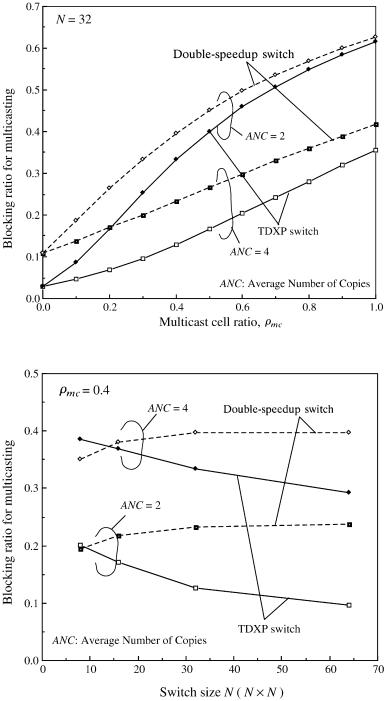
Figures 9.9 and 9.10 show the blocking ratio Bblock for multicasting traffic. Bblock is defined as the ratio of the offered input cells to the cells not transmitted from the input buffer on account of HOL blocking. In this case,
the offered input traffic load is set to 1.0. The multicast mechanism employed
is that presented in Section 9.2.3. The Bblock of the TDXP switch is smaller than that of the double-speedup switch with N s 32. The reason is as
follows. In the double-speedup switch, if at least one of the destination output ports is occupied by another cell belonging to a different input port, the multicast cell is blocked at the HOL in the input buffer. On the other hand, in the TDXP switch, even when the destined output ports are so occupied, the cell is buffered in the tandem crosspoint, and an attempt is made to send it through the next switch plane in the next time slot. Therefore, the following multicast cell in the input buffer can be transmitted to all destination tandem crosspoints as long as none of them is buffering a cell. This benefit of the TDXP switch is large when N is large and the average number of copies ŽANC. is small in other words, NrANC is large
as shown in Figure 9.10. However, if NrANC is small, Bblock of the TDXP switch is higher than that of the double-speedup switch. For example, we can
see such a case with N F 15 and ANC s 4.
PERFORMANCE OF TDXP SWITCH |
251 |
Fig. 9.9 Blocking ratio for multicasting.
Fig. 9.10 Blocking ratio for multicasting vs. switch size and average number of copies.
252 THE TANDEM-CROSSPOINT SWITCH
REFERENCES
1.G. Balboni, M. Collivignarelli, L. Licciardi, A. Paglialunga, G. Rigolio, and F. Zizza, ‘‘From transport backbone to service platform: facing the broadband switch evolution,’’ Proc. ISS ’95, pp. 26, 1995.
2.T. Chaney, J. A. Fingerhut, M. Flucke, and J. S. Turner, ‘‘Design of a gigabit ATM switch,’’ Proc. IEEE INFOCOM ’97, pp. 2 11, 1997.
3. M. Collivignarelli, A. Daniele, P. De Nicola, L. Licciardi, M. Turolla, and A. Zappalorto, ‘‘A complete set of VLSI circuits for ATM switching,’’ Proc. IEEE GLOBECOM ’94, pp.134 138, 1994.
4.K. Genda, Y. Doi, K. Endo, T. Kawamura, and S. Sasaki, ‘‘A 160-Gbrs ATM switching system using an internal speed-up crossbar switch,’’ Proc. IEEE GLOBECOM ’94, pp. 123 133, 1994.
5.M. J. Karol, M. G. Hluchyj, and S. P. Morgan, ‘‘Input versus output queueing on a space-division packet switch,’’ IEEE Trans. Commun., vol. COM-35, pp. 1347 1356, Dec. 1987.
6.T. Kawamura, H. Ichino, M. Suzuki, K. Genda, and Y. Doi, ‘‘Over 20 Gbitrs throughput ATM crosspoint switch large scale integrated circuit using Si bipolar technology,’’ Electron. Lett., vol. 30, pp. 854 855, 1994.
7.L. Licciardi and F. Serio, ‘‘Technical solutions in a flexible and modular architecture for ATM switching,’’ Proc. Int. Symp. Commun. Ž ISCOM ’95., pp. 359 366, 1995.
8.P. Newman, ‘‘A fast packet switch for the integrated services backbone network,’’ IEEE J. Select. Areas Commun., vol. 6, pp.1468 1479. 1988.
9.Y. Oie, M. Murata, K. Kubota, and H. Miyahara, ‘‘Effect of speedup in nonblocking packet switch,’’ Proc. IEEE ICC ’89, p. 410, 1989.
10.Y. Oie, T. Suda, M. Murata, D. Kolson, and H. Miyahara, ‘‘Survey of switching techniques in high-speed networks and their performance,’’ Proc. IEEE INFO- COM ’90, pp. 1242 1251, 1990.
11.E. Oki, N. Yamanaka, and S. Yasukawa,‘‘Tandem-crosspoint ATM switch architecture and its cost-effective expansion,’’ IEEE BSS ’97, pp. 45 51, 1997.
12.E. Oki and N. Yamanaka, ‘‘A high-speed tandem-crosspoint ATM switch architecture with input and output buffers,’’ IEICE Trans. Commun., vol. E81-B, no. 2, pp. 215 223, 1998.
13.J. S. Turner, ‘‘Design of a broadcast packet switching networks,’’ IEEE Trans. Commun., vol. 36, pp. 734 743, 1988.
14.N. Yamanaka, K. Endo, K. Genda, H. Fukuda, T. Kishimoto, and S. Sasaki, ‘‘320 Gbrs high-speed ATM switching system hardware technologies based on copperpolyimide MCM,’’ IEEE Trans. CPMT, 1996, vol.18, pp. 83 91, 1995.

Broadband Packet Switching Technologies: A Practical Guide to ATM Switches and IP Routers
H. Jonathan Chao, Cheuk H. Lam, Eiji Oki
Copyright 2001 John Wiley & Sons, Inc. ISBNs: 0-471-00454-5 ŽHardback.; 0-471-22440-5 ŽElectronic.
CHAPTER 10
CLOS-NETWORK SWITCHES
In Chapter 6 and Chapter 7, we have studied how to recursively construct a large switch from smaller switch modules based on the channel grouping principle. In such a construction, every input is broadcast to each first-stage module, and the input size of first-stage modules is still the same as that of the entire switch.
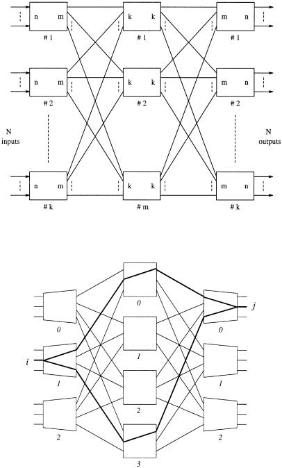
In this chapter we consider a different approach to build modular switches. The architecture is based on the Clos network Žsee Fig. 10.1.. Switch modules are arranged in three stages, and every module is interconnected with every module in the adjacent stage via a unique link. In this book, the three stages are referred as input stage, middle stage, and output stage, respectively. The modules in those stages are accordingly called input modules, central modules, and output modules. Each module is assumed to be nonblocking and could be, for example, one of the crossbar switches described previously. Inputs are partitioned into groups, and only one group of inputs are connected to each input module, thereby reducing the size of each module.
One may wonder why we are not just considering a two-stage interconnection network in which every pair of modules of adjacent stages are interconnected with a dedicated link. In that case, no two cells can be simultaneously transmitted between any pair of modules, because there is just one path between them. In a Clos network, however, two cells from an input module can take distinct paths via different central modules to get to the same module at the output stage Žsee Fig. 10.2.. The central modules in the middle stage can be looked on as routing resources shared by all input and output modules. One can expect that this will give a better tradeoff between the switch performance and the complexity.
253
254 CLOS-NETWORK SWITCHES
Fig. 10.1 A growable switch configuration.
Fig. 10.2 Routing in a Clos network.
ROUTING PROPERTIES AND SCHEDULING METHODS |
255 |
Because of this desirable property, the Clos network was widely adopted in traditional circuit-switched telephone networks, where a path is reserved in the network for each call. If a Clos network has enough central modules, a path can always be found for any call between an idle input and an idle output. Such a property is called nonblocking. There are however two senses of nonblocking: strict and rearrangeable. In a strictly nonblocking Clos network, every newly arriving call will find a path across the network without affecting the existing calls. In a rearrangeably nonblocking network, we may have to arrange paths for some existing calls in order to accommodate a new arrival. Readers are encouraged to learn more about circuit-switched Clos networks from the related references listed at the end of this chapter.
This chapter will then focus on how the Clos network is used in packet switching. Section 10.1 describes the basic routing properties in a Clos network and formulates the routing as a scheduling problem. In the following sections, we will discuss several different scheduling approaches. Section 10.2 uses a vector for each input and output module to record the availability of the central modules. Those vectors are matched up in pairs, each of which has one vector for an input module and the other for an output module. For those pairs of modules that have a cell to dispatch between them, the two vectors will be compared to locate an available central module if any. This method is conceptually easy, but it requires a high matching speed. In Section 10.3, the ATLANTA switch handles the scheduling in a distributed manner over all central modules, each of which performs random arbitration to resolve the conflicts. Section 10.4 describes a concurrent dispatching scheme that does not require internal bandwidth expansion while achieving a high switch throughput. The path switch in Section 10.5 adopts the quasi-static virtual-path routing concept and works out the scheduling based on a predetermined central stage connection pattern, which may be adjusted when the traffic pattern changes. All of these will give us different viewpoints to look at the tradeoff between scheduling efficiency and complexity in a packet-switched Clos network.
10.1ROUTING PROPERTIES AND SCHEDULING METHODS
A three-stage Clos network is shown in Figure 10.1. The first stage consists of k input modules, each of dimension n m. The dimension of each central module in the middle stage is k k. As illustrated in Figure 10.2, the routing constraints of Clos network are briefly stated as follows:
1.Any central module can only be assigned to one input of each input module, and one output of each output module;
2.Input i and output j can be connected through any central module;
3.The number of alternative paths between input i and output j is equal to the number of central modules.
256 CLOS-NETWORK SWITCHES
For the N N switch shown in Figure 10.1, both the inputs and the outputs are divided into k modules with n lines each. The dimensions of the input and output modules are n : m and m : n, respectively, and there are m middle-stage modules, each of size k k. The routing problem is one of directing the input cells to the irrespective output modules without path conflicts. For every time slot, the cell traffic can be written as
|
|
t1, 1 |
t1, 2 |
|
t1, k |
|
|
|
. |
. |
|
. |
|
|
|
T s |
. |
. |
|
. |
|
, |
|
. |
. |
|
. |
|
|||
|
|
tk , 1 |
tk , 2 |
|
tk , k |
|
|
where ti, j represents the number of cells arriving at the ith input module destined for the jth output module. The row sum is the total number of cells arriving at each input module, while the column sum is the number of cells destined for each output module, and they are given by
k
Ri s Ý ti , j js1
k
Sj s Ý ti , j is1
F n F m, i s 1, 2, . . . , k, |
Ž10.1. |
F n, j s 1, 2, . . . , k. |
Ž10.2. |
Since at most m cells for each output group are considered, the column sum constraint can then be rewritten as
Sj F m, j s 1, 2, . . . , k. |
Ž10.3. |
The routing requirement is to assign each cell a specific path through the first two stages such that no two cells from an input module will leave at the same outlet of the input module, and no two cells destined for the same output module will arrive at the same inlet of the output module. Such an assignment is guaranteed by the nonblocking property of the three-stage Clos network for m G n.
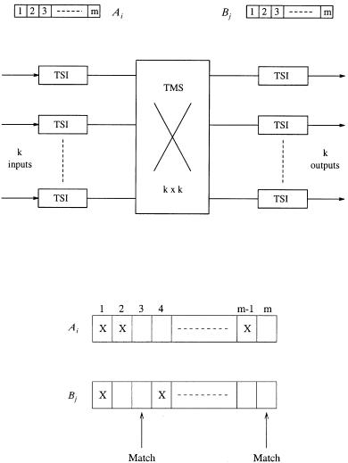
Let us label the set of outlets from each input module by Ai Ži s 1, . . . , k. and the set of inlets into each output module by Bj Ž j s 1, . . . , k.. Each Ai or Bj contains exactly m elements denoting m physical lines. If these elements are viewed as time slots instead of physical lines, then the first two stages can be transformed into a k k time space time ŽTST. switch Žsee Figure 10.3., where each input frame Ž Ai . and output frame Ž Bj . has m slots. The assignment problem is now seen as identical to that of a classic TST switch, and the necessary and sufficient conditions to guarantee a perfect or optimal schedule are satisfied by Ž10.1. and Ž10.3. w3x. For the assignment of an arbitrary cell at a given input module to its output module, the status of its
ROUTING PROPERTIES AND SCHEDULING METHODS |
257 |
Fig. 10.3 A TST switch representation after the space-to-time transformation. Ž 1992 IEEE..
Fig. 10.4 Matching of Ai and Bj ŽX s busy, blank s open.. Ž 1992 IEEE..
Ai and the corresponding Bj may be examined, as shown in Figure 10.4, where any vertical pair of idle slots Žrepresenting physical lines. could be chosen as a valid interconnect path. An overall schedule is perfect if all cells are successfully assigned without any path conflict. However, optimal scheduling requires global information on the entire traffic T, and the implementation tends to be very complex.