Biomechanics Principles and Applications - Donald R. Peterson & Joseph D. Bronzino

These equations can be solved numerically for the case of a step change in acceleration or velocity of the skull [Grant and Cotton, 1991]. Solutions for both step change in acceleration and velocity are shown in Figure 18.3.

18.5 Otolith Transfer Function

A transfer function of otoconial layer deflection re. (related to) skull acceleration can be obtained from the governing equations [Grant et al., 1994]. Starting with the nondimensional fluid and gel layer equations, taking the Laplace transform with respect to time and using the initial conditions, gives two ordinary differential equations. These equations can then be solved using the boundary conditions. Taking the Laplace transform of the otoconial layer motion equation, combining with the two differential equation solutions, and integrating otoconial layer velocity to get deflection produces the transfer function for displacement re. acceleration

s is the Laplace transform variable, and a general acceleration term A is defined as

18.6 Otolith Frequency Response

This transfer function can now be studied in the frequency domain. It should be noted that these are linear partial differential equations and that the process of frequency domain analysis is appropriate. The range of values of ε = 0.01 to 0.2, M = 5 to 20, and R = 0.75 have been established [Grant and Cotton, 1991] in a numerical finite difference solution of the governing equations. Having established these values the frequency response can be completed.

In order to construct a magnitude and phase vs. frequency plot of the transfer function, the nondimensional time will be converted back to real time for use on the frequency axis. For the conversion to real time the following physical variables will be used: ρo = 1350 kg/m3, b = 15μm, and μf = 0.85 mPa/sec. The general frequency response is shown in Figure 18.4. The flat response from DC up to the first corner frequency establishes this system as an accelerometer. This is the range of motion frequencies encountered in normal motion environments where this transducer is expected to function.

The range of flat response can be easily controlled with the two parameters and ε and M. It is interesting to note that both the elastic term and the system damping are controlled by the gel layer, thus an animal can easily control the system response by changing the parameters of this saccharide gel layer. The crosslinking of saccharide gels is extremely variable yielding vastly different elastic and viscous properties of the resulting structure. The density ratio R has the effect of changing the magnitude of the response, and the parameters ε and M control the dynamics of the response.

The otoconial layer transfer function can be compared to recent data from single fiber neural recording. The only discrepancy between the experimental data and theoretical model is a low-frequency phase lead and accompanying amplitude reduction. This has been observed in most experimental single-fiber recordings and has been attributed to the hair cell.

18.7 Semicircular Canal Distributed Parameter Model

The membranous SCC duct is modeled as a section of a rigid torus filled with an incompressible Newtonian fluid. The governing equations of motion for the fluid are developed from the Navier-Stokes equation. Refer to the nomenclature section for definition of all variables, and Figure 18.5 for a cross section of the SCC and membranous utricle sack.

Semicircular Canal Variables

α= angular acceleration of the canal wall measured with respect to an inertial frame

ω= angular velocity of the canal wall measured with respect to an inertial frame

φ= angular displacement of the canal wall measured with respect to an inertial frame

= magnitude of a step change of angular velocity of the head or canal wall

β= angle subtended by the canal in radians (β = π for a true semicircular canal)

We are interested in the flow of endolymph fluid with respect to the duct wall and this requires that the inertial motion of the duct wall R be added to the fluid velocity u measured with respect to the duct wall. The curvature of the duct can be shown to be negligible since a R, and no secondary flow is

a

r

SCC duct

Duct cross section

R

Cupula

Crista

Utricle

FIGURE 18.5 Schematic structure of the semicircular canal showing a cross section through the canal duct and utricle. Also shown in the upper right-hand corner is a cross section of the duct. R is the radius of curvature of the semicircular canal, a is the inside radius to the duct wall, and r is the spatial coordinate in the radial direction of the duct.

induced, thus the curve duct can be treated as straight. Pressure gradients arise from two sources in the duct

(1) presence of the utricle and (2) from the cupula. The cupula, when deflected, exerts a restoring force on the endolymph. The cupula can be modeled as a membrane with a linear pressure–volume modulus K = p/ V , where p is the pressure difference across the cupula, which is produced by a volumetric displacement V , where

If the angle subtended by the membranous duct is denoted by β, the pressure gradient in the duct produced by the cupula is

The utricle pressure gradient can be approximated by [Van Buskirk, 1977]

When this information is substituted into the Navier-Stokes equation the following governing equation for endolymph flow relative to the duct wall is obtained

This equation can be nondimensionalized using the following nondimensional variables denoted by overbars

In terms of the nondimensional variables the governing equation for endolymph flow velocity becomes

which contains physical parameters for the system mass, stiffness, and damping. This ε parameter governs the response of the canals to angular acceleration. The boundary and initial conditions for this equation are as follows

18.8 Semicircular Canal Frequency Response

To examine the frequency response of the SCC, a transfer function must be developed that relates the mean angular displacement of endolymph to head motion. The objective of this analysis is to see if the SCCs are angular acceleration, velocity, or displacement sensors. To achieve this, a relationship between α = angular acceleration, ω = angular velocity, and φ = angular displacement of the head, all measured

with respect to an inertial reference frame, is developed. This relationship in terms of the Laplace transform variable s is

To relate these to the mean angular displacement of endolymph, the volumetric displacement V = 0t ( 0a (u(r, t)2π r dr ))dt is calculated from the distributed parameter solution and this is related to the

mean angular displacement of the endolymph θ as

Using the solution to the distributed parameter formulation for the SCC, for ε 1, and for a step change in angular velocity of the canal wall , the volumetric displacement becomes

where λn represents the roots of the equation J 0(x) = 0, where J 0 is the Bessel function of zero order (λ1 = 2.405, λ2 = 5.520, . . .) [Van Buskirk et al., 1976; Van Buskirk and Grant, 1987].

A transfer function in terms of s can now be developed for frequency response analysis. This starts by developing an ordinary differential equation in θ for the system, using a moment sum about the SCC center, and developing terms for the inertia, damping, restoring moment created by the cupula incorporatingV . Using this relationship and Equation 18.20, the transfer function of mean angular displacement of

where the two time constants, one long (τL) and one short (τs) are given by:

where τL τS. Here the angular velocity of the head is used instead of the angular acceleration or angular displacement because, in the range of frequencies encountered by humans in normal motion, the canals are angular velocity sensors. This is easily seen if the other two transfer functions are plotted.

The utility of the above transfer function is apparent when used to generate the frequency response of the system. The values for the various parameters for humans are as follows: a = 0.15 mm, R = 3.2 mm, the dynamic viscosity of endolymph μ = 0.85 mPa sec, ρf = 1000 kg/m3, β = 1.4π , and K = 3.4 GPa/m3. This produces values of the two time constants of τL = 20.8 sec and τs = 0.00385 sec. The frequency response of the system is shown in Figure 18.6. The range of frequencies from 0.01 to 30 Hz establishes the SCCs as angular velocity transducers of head motion. This range includes those encountered in everyday movement. Environments such a aircraft flight, automobile travel, and shipboard travel can produce frequencies outside the linear range for these transducers.

Rabbitt and Damino [1992] have modeled the flow of endolymph in the ampulla and its interaction with the cupula. This model indicates that the cupula adds a high frequency gain enhancement as well as phase lead over previous mechanical models. This is consistent with measurements of vestibular nerve recordings of gain and phase. Prior to this work, this gain and phase enhancement were thought to be of hair cell origin.

SCC transfer function

(a) 10–2

Frequency, Hz

(b)100

50

Frequency, Hz

FIGURE 18.6 Frequency response of the human semicircular canals for the transfer function of mean angular displacement of endolymph fluid θ re. angular velocity of the head ω.

18.9 Hair Cell Structure and Transduction

As can be seen from the two frequency response diagrams for the otolith and SCC, the sensed variables, linear acceleration in the case of the otolith and angular velocity for the SCC, are transduced into a displacements. These displacements are cupula displacement for the SCC and otoconial layer displacement for the otolith. These displacements are then further transduced into neural signals by the hair cells in each sensory organ. The hair cells project small cilia or hairs, called stereocilia, from the apical surface of the cell body into the otolith gel layer and cupula (see Figure 18.7 and Figure 18.8). Figure 18.7 shows the geometry of a single stereocilium, which is cylindrical in shape and has a tapered base. Each stereocilium has an internal core of actin, which deforms when a force is applied to its top. Because of the tapered base, most of the deformation in a stereocilium is bending in this tapered section with a top force applied. Both bending and shear deformation take place throughout the entire stereocilia when they are deflected.

The stereocilia of a single hair cell form a bundle, with definite regular spacing in an hexagonal array when viewed from the top (see Figure 18.7). The height of each stereocilium in a bundle increases, in a stepwise fashion, to form an organ pipe arrangement. Stereocilia in a bundle are bound together by a set of links the run from stereocilia to stereocilia. These bundle links are what forms a bundle into a single functional unit. These links come in many types; however, there are two main structural types, tip links that run up at an angle from the tip of the stereocilia to its next taller neighbor, and upper lateral links that run horizontally in sets. The lateral links extend from one stereocilia to its six neighbors, forming six sets associated with each stereocilia.

A set is composed of a group of links that are spaced up and down the height of the stereocilia. The protein composition of these links is unknown, but each type of link is believed to have a different structure. The tip links are stiff and resist elongation more than the lateral links. The tallest cilia in the bundle is called a kinocilium, which is a true cilia with 9+2 tubule structure, different from the stereocilia, and it is linked to its neighboring stereocilia by a third type of link called a stereocilia–kinocilium link. Other link

Lateral link

Tip links—top view

(e)

Lateral links—top view

Links—lateral view

FIGURE 18.7 Configuration of a vestibular hair cell bundle. (a) Stereocilia geometry of circular shaft with tapered base. These stereocilia are composed of actin surrounded by the cell membrane. (b) Bundle geometry for a typical vestibular stereocilia bundle, showing the staircase arrangement of increasing height of the stereocilia in the bundle. The tallest cilia in the bundle is different in structure from the stereocilia and is called a kinocilium, which has the 9+2 microtubule structure of a true cilium. The microtubule structure lacks the biochemical ability to be mobile and it appears to be present for structural rigidity only. (c) Lateral view of two stereocilia connected by tip and lateral links.

(d) Top view of the stereocilia showing the locations of orientation of the tip links. (e) Top view of the stereocilia showing the locations and orientation of the lateral links.

structures have been identified in the bundle but will not be discussed here, as these are thought to be insignificant structural links. These interconnected stereocilia and kinocilium form a complete vestibular bundle.

Kinocilia are attached to the cupula and otoconial gel layer so that when these are deflected the kinocilia are also deflected pulling the entire hair cell bundle with it. When a hair cell bundle is deflected by a force applied to the kinocilium in a direction away from the bundle, the resulting deflection stretches the tip

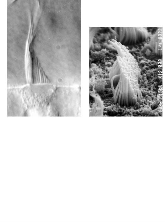
FIGURE 18.8 Photomicrographs of real hair cell bundles. (a) Light micrograph (DIC). (b) Scanning electron microscope of a bundle in the striolar region of the utricle (×12,000). Due to the fixation and drying for electron microscopy many artifacts are introduced in the bundle. (Photomicrographs taken by Dr. Ellengene Peterson, Ohio University, and used here with permission.)

links increasing their tension. In addition, lateral links are tensioned as well. The increased tension in a tip link increases the probability that an ion channel attached to the tip link will open. These ion channels are imbedded in the outer lipid bilayer of the hair cell and there is evidence that there are as many as two channels on each tip link. When tip link tension opens a channel, it allows free positive ions from the surrounding endolymph fluid to flow into the intercellular space of the hair cell. This influx of positive ions decreases the resting membrane potential of the cell. This starts the cascade of events that are associated with the depolarization of any sensory receptor cell, which ends with the release of neurotransmitter, and firing of the nerve that is in contact with the cell. In this fashion the mechanical deflection of the hair cell’s bundle is converted into a neural signal. This process is termed mechanotransduction, and when linked with the extracellular structure of otoconial layer deflection and cupula deflection, the entire organ function becomes a complex inertial motion sensor of the head.

18.10 Hair Cell Mechanical Model

Mechanical deformation behavior of the hair cell bundles has been analyzed using finite element analysis (FEA). This analysis was done using a custom-written program that will accommodate any hair bundle configuration [Cotton and Grant, 2000]. The resulting model is a three-dimensional, distributed parameter formulation that ramps up any applied force in incremental steps. Each force step considers the new, deformed geometry and recalculates displacements, link tensions, and internal force directions, until each of these values converges. This incremental ramp loading is a nonlinear computational process.

1.6 1.6 N

2. 2.7 3.6 3.8 3.7 N

2.5 3.1 3.9 5.1 7.3 8.8 N

2.8 3.4 3.3 N

FIGURE 18.9 Circle plots of a bundle showing the tip link tensions in pN. These plots are topviews of the bundle where each stereocilia and kinocilium in the bundle is represented by a circle. The arrangement is to scale and represents the organization of cilia studied. The tip links are represented as solid lines connecting the circles. The number inside each circle represents the tension in the tip link attached to the top of that stereocilium that runs to the side of the next taller stereocilium. The shading is a relative designation of the tip link tension within that bundle, with dark indicating maximum tension. Stereocilia with an N designation indicates the absence of a tip link due to the absence of a taller stereocilium for attachment. The kinocilium is shown with a K in its circle. In the figure the bundle has a point loaded force applied at the top of the kinocilium. The magnitude of the applied force was adjusted to produce a bundle deflection of 50 nm. The force magnitude to produce the 50 nm deflection is 8 pN.

The model uses shear deformable beam elements for cilia. Tip links and lateral links are modeled as two-force members with linear spring-like behavior in tension. Lateral links can buckle and are not allowed to support compressive loads. Tip links are almost always in tension, they are treated similarly to lateral links, and are not allowed to support a compressive load.

The program allows input specifications of material and geometric properties. Geometric properties include cilia and link diameters, tapering at the base of stereocilia, and cilia locations on the hair cell’s apical surface. Material properties include elastic moduli for cilia and links, and the shear moduli for cilia.

In order to formulate a realistic bundle model, geometric data was gathered using light microscope and SEM photomicrographs. Material properties were determined from reference materials and using parametric studies. Figure 18.9 illustrates the pattern of tip link tensions generated in a bundle that is loaded with a force of sufficient magnitude to produce a 50-nm deflection, a typical large physiologic deflection (for details see Silber et al., 2004). In this figure, circles represent the configuration of stereocilia and kinocilium (K) on the apical surface of each hair cell (bundle viewed from top). The number inside each circle is the magnitude of tension in pN (peco Newtons) for the tip link attached to the top of that stereocilium; shading is scaled to this magnitude. The simulations shows that tensions are highest close to the kinocilium, and they drop steadily with distance from the kinocilium. Note also that higher tensions generally tend to occur in the middle columns of the bundle; peripheral columns have relatively low tensions, even those close to the kinocilium.

18.11 Concluding Remark

The mechanical signal of inertial head motion has been followed and quantified through the vestibular organs to neural signals that are generated in the receptor hair cells. As stated in the introduction, the central nervous system uses these signals for eye positioning during periods of motion and to coordinate muscular activity. The biggest problem for people who have lost their vestibular function is not being able to see during periods of body motion. Implantable artificial vestibules are being developed for future medical application.

References

Cotton, J.R. and Grant, J.W. 2000. A finite element method for mechanical response of hair cell ciliary bundles. J. Biomech. Eng., Trans. ASME 122: 44–50.

Grant, J.W., Huang, C.C., and Cotton, J.R. 1994. Theoretical mechanical frequency response of the otolith organs. J. Vestib. Res. 4: 137–151.

Grant, J.W. and Cotton, J.R. 1991. A model for otolith dynamic response with a viscoelastic gel layer.

J. Vestib. Res. 1: 139–151.

Grant, J.W., Best, W.A., and Lonegro, R. 1984. Governing equations of motion for the otolith organs and their response to a step change in velocity of the skull. J. Biomech. Eng. 106: 302–308.

Rabbitt, R.D. and Damino, E.R. 1992. A hydroelastic model of macromechanics in the endolymphatic vestibular canal. J. Fluid Mech. 238: 337–369.

Silber, J., Cotton, J., Nam, J., Peterson, E., and Grant, W. 2004. Computational models of hair cell bundle mechanics: III. 3-D utricular bundles. Hearing Res. (in press).

Van Buskirk, W.C. and Grant, J.W. 1987. Vestibular mechanics. In Handbook of Bioengineering, Eds. R. Skalak and S. Chien, pp. 31.1–31.17. McGraw-Hill, New York.

Van Buskirk, W.C. 1977. The effects of the utricle on flow in the semicircular canals. Ann. Biomed. Eng. 5: 1–11.

Van Buskirk, W.C., Watts, R.G., and Liu, Y.K. 1976. Fluid mechanics of the semicircular canal. J. Fluid Mech. 78: 87–98.