Genomics and Proteomics Engineering in Medicine and Biology - Metin Akay

26 INTERPRETING MICROARRAY DATA AND RELATED APPLICATIONS

given only access to the system inputs and outputs gathered experimentally. The methods are sometimes called “nonparametric” because they do not assume a detailed model structure such as that the inputs and outputs are related through a set of differential equations, where only certain parameter values need to be ascertained. Indeed, virtually no a priori knowledge of the system’s structure is assumed, rather the system is regarded as an impenetrable blackbox. We consider only such methods because we will view the interpretation of gene expression profiles as essentially a case where the expression levels give rise to input signals, while the classes of importance, such as metastatic and nonmetastatic or failed outcome and survivor, create the desired output signals. The desired class predictor results from identifying a nonlinear system that is defined only by these input and output signals.

Throughout this chapter, it will be assumed that the given nonlinear system is time invariant, namely that a translation of the system inputs in time results in a corresponding translation of the system outputs. Such an assumption causes no difficulty in applying the approach to class prediction. One celebrated blackbox approach assumes that the input–output relation can be well approximated by a functional expansion such as the Volterra [1, 2] or the Wiener series [3]. For example, for the case of a single input x(t) and single output y(t), the approximation has form

and e(t) is the model error. The right side of Eq. (2.2) is a Jth-order Volterra series with memory length T and the weighting function hj is called the jth-order Volterra kernel. The zero-order kernel h0 is a constant. System identification here reduces to estimation of all of the significant Volterra kernels, which involves solution of a set of simultaneous integral equations and is usually a nontrivial task. A fairly narrow class of systems, known as analytic [1, 2], can be exactly represented by the Volterra series of Eq. (2.2), where both J and T could be infinite. However, a much wider class can be uniformly approximated by such a series, with both J and T finite, according to Fre´chet’s theorem [4], which has been extended by Boyd and Chua [5]. The essential requirements are that the nonlinear system must have either finite [4] or fading [5] memory, and its output must be a continuous mapping of its input, in that “small” changes in the system input result in small changes in the system output. Then, over a uniformly bounded, equicontinuous set of input signals, the system can be uniformly approximated, to any specified degree of accuracy, by a Volterra series of sufficient but finite order J.

Wiener [3] essentially used the Gram–Schmidt process to rearrange the Volterra series into a sum of terms that were mutually orthogonal for a white Gaussian input x

with a specified power density level. The mutually orthogonal terms in Wiener’s functional expansion were called G-functionals (G for Gaussian). The advantage of creating orthogonal functionals was to simplify kernel estimation and remove the requirement of solving simultaneous integral equations. Indeed, Wiener kernels in this expansion were determinable using the cross-correlation formula of Lee and Schetzen [6]. The Wiener kernels are not, in general, the same as the Volterra kernels, but when the complete set of either is known, the other set can be readily computed. If a system can be represented exactly by a second-order Volterra series [i.e., e(t) ; 0 in Eq. (2.1) and J ¼ 2 in Eq. (2.2)], then the firstand second-order Volterra kernels equal the Wiener kernels of corresponding order. Once the kernels have been estimated, Eq. (2.2) can be used to calculate the Volterra series output for an arbitrary input x and thus “predict” the actual output y of the given nonlinear system.

In discrete time, for single input x(i) and single output y(i), the approximation has form

and e(i) is the model error. The Dth-order Volterra series on the right side of Eq. (2.4) has memory length R þ 1 because z(i) depends not only on x(i) but also on earlier values x(i), . . . , x(i R), that is, at input lags 0, . . . , R.

Indeed, this discrete-time Volterra series is simply a Dth-degree multidimensional polynomial in x(i), . . . , x(i R), and the kernels hd( j1, . . . , jdÞ, d ¼ 0, . . . , D, are directly related to the coefficients of this polynomial. The zeroorder kernel h0 is the constant term of the polynomial. Any discrete-time system of finite [7] or fading memory whose output is a continuous mapping of its input (in the sense described above) can be uniformly approximated, over a uniformly bounded set of input signals, by the Volterra series on the right side of Eq. (2.4). Of course, D and R must be sufficiently large (but finite) to achieve the desired degree of accuracy. Applying the Gram–Schmidt process to the terms on the right side of Eq. (2.4) for a white Gaussian input x of specified variance can create a discrete form of the Wiener series. The kernels in this Wiener series are directly related to the Volterra kernels, and once the complete set of either is known, the other set can be readily calculated.

Several methods are available for estimating the Wiener or the Volterra kernels. If the input x is white Gaussian, then the Wiener kernels can be estimated using cross correlation either directly in the time domain by the Lee–Schetzen method [6] or efficiently in the frequency domain via the method of French and Butz [8]. The Lee–Schetzen approach was actually presented in continuous time [6] but is now most commonly applied in discrete time. Amorocho and Brandstetter [9], and later

28 INTERPRETING MICROARRAY DATA AND RELATED APPLICATIONS

Watanabe and Stark [10] and Marmarelis [11], expanded the kernels using Laguerre functions, then least-squares estimated the coefficients in the resulting expansion, and finally reconstructed the kernels using the estimated coefficients. Ogura [12] noted that use of Laguerre functions to approximate kernels having initial delay was less accurate than employing “associated” Laguerre functions and developed a fast algorithm for calculating the outputs of biorthogonal Laguerre filters.

Alternatively, the fast orthogonal algorithm (FOA) [13, 14] can be employed to estimate either the Wiener or the Volterra kernels, as can parallel cascade identification [14, 15]. Very widespread use has been made of the Lee–Schetzen [6] technique, with Sandberg and Stark [16] and Stark [17] being some of the first to exploit its power in modeling the pupillary control system. Marmarelis and Naka [18] and Sakai and Naka [19, 20] made imaginative applications of the Lee–Schetzen [6] technique to study information processing in the vertebrate retina. Barahona and Poon [21] used the FOA to detect deterministic nonlinear dynamics in short experimental time series. Orcioni et al. [22] studied the Lee–Schetzen [6] and fast orthogonal [13, 14] algorithms and gave practical suggestions concerning optimal use of these methods for estimating kernels up to third order. Zhang et al. [23] proposed a method of combining Akaike’s final prediction error criterion [24, 25] with the FOA [13, 14] to determine the memory length simultaneously with the kernels. Westwick et al. [26] developed bounds for the variance of kernel estimates, computable from single data records, for the FOA [13, 14] and for kernel estimation via use of Laguerre functions [9–12].

When different kernel estimation procedures are compared, an issue that is sometimes overlooked is whether the test system’s kernels are smooth or, instead, jagged and irregular. Smooth kernels can usually be well approximated using a small number of suitably chosen basis functions, such as the Laguerre set; jagged kernels typically cannot. If the simulated test system has smooth kernels, this favors basis expansion methods for estimating kernels, because they will require estimation of far fewer parameters (the coefficients in a brief basis function expansion) than the set of all distinct kernel values estimated by the FOA. In those circumstances, basis expansion methods will be shown in their best light, but a balanced presentation should point out that the situation is quite different when the test kernels have jagged or irregular shapes. Indeed, one may overlook valuable information inherent in the shape of a system’s kernels by assuming a priori that the kernels are smooth. Moreover, in some applications, for example, Barahona and Poon’s [21] use of functional expansions to detect deterministic dynamics in short time series, restrictive assumptions about the kernels’ shapes must be avoided. If it cannot be assumed that the kernels are smooth, then the basis function approach will generally require an elaborate expansion with many coefficients of basis functions to be estimated. Hence the FOA is advantageous because it exploits the lagged structure of the input products on the right side of Eq. (2.4) to dramatically reduce computation and memory storage requirements compared with a straightforward implementation of basis expansion techniques.

The FOA uses the observation that estimating least-squares kernels up to Dth order in Eq. (2.4) requires calculating the input autocorrelation only up to order

2D 1. For example, suppose that the system input x(i) and output y(i) are available for i ¼ 0, . . . , I and that we seek the best approximation of the output, in the leastsquares sense, by a second-order Volterra series [D ¼ 2 in Eq. (2.4)]. Then this requires calculating the input mean and autocorrelations up to third order, namely

The lower order autocorrelations are defined analogously. For I . R3, the most time-consuming part of the FOA is the calculation of the third-order autocorrelation. The computational requirement to do this has been overestimated in various publications (e.g. [27]), sometimes three times too large, so it is worthwhile to consider an efficient scheme. For example, the input mean and thirdand lower order autocorrelations can be obtained as follows:

For i = R to I Q = x(i)

Avg = Avg + Q

For i1 = 0 to R QQ = Q.x(i-i1)

fxx(i1)= fxx(i1) + QQ For i2 = 0 to i1 QQQ = QQ.x(i-i2)

fxxx(i1,i2) = fxxx(i1,i2) + QQQ For i3 = 0 to i2

QQQQ = QQQ.x(i - i3)

fxxxx(i1,i2,i3)= fxxxx(i1,i2,i3)+ QQQQ Next i3

Next i2 Next i1

Next i

After this, each of Avg, fxx, fxxx, fxxxx is divided by I R þ 1. The above pseudocode requires about IR3=3! multiplications to compute the mean and all autocorrela-

tions up to third order [14], and for I . R3, that is the majority of multiplications the FOA requires to calculate kernels up to second order.

For the most part, Volterra [1, 2] and Wiener [3] series are of practical use for approximating “weakly nonlinear” systems, with an order of nonlinearity less than or equal to, say, 3. In instances where it is possible to precisely apply special inputs, for example complete binary m-sequences, then high-order kernels can be rapidly and accurately estimated by Sutter’s innovative approach [28, 29]. Alternatively, some nonlinear systems can be well approximated by a cascade of a dynamic

30 INTERPRETING MICROARRAY DATA AND RELATED APPLICATIONS

linear, a static nonlinear, and a dynamic linear element [30–33], sometimes referred to as an LNL cascade. A method that leads to an identification of each of these elements, within arbitrary scaling constants and a phase shift, from a single application of a white Gaussian noise input was presented in 1973 [32, 33] and has had several applications in neurophysiology [34–36]. One interesting property of the LNL cascade is that its Wiener kernels are proportional to its Volterra kernels of corresponding order [32, 33]. Moreover, for a white Gaussian input, the shape of the first linear element’s impulse response is given by the first nonnegligible slice of a second-order cross correlation parallel to one axis [15, 37]. Thus the

first nonnegligible term in the sequence fxxy( j, 0), fxxy( j, 1), . . . (here fxxy is the second-order cross correlation between a white Gaussian input xðiÞ and the

cascade output yðiÞ after removing its mean) reveals the first dynamic linear element up to a scaling constant. Subsequently, methods related to the approach of [32, 33] have been published by a number of authors [15, 37–39]. However, the use of such inputs does not apply to the case of interpreting gene expression profiles. For the latter application, it is useful to resort to parallel cascade identification [14, 15], which is effective in approximating systems with high-order nonlinearities and does not require special properties of the input.

2.3. PARALLEL CASCADE IDENTIFICATION

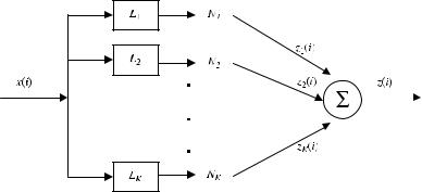
Parallel cascade identification (PCI) seeks to approximate a given discrete-time dynamic nonlinear system by building a parallel array of alternating dynamic linear (L) and static nonlinear (N) elements using only the system’s input–output data gathered experimentally [14, 15]. By “dynamic” is meant that the element has memory of length R þ 1, as explained above, where R . 0. An example of a parallel LN cascade model is shown in Figure 2.1 and will be used below for class prediction. This parallel LN model is related to a parallel LNL model introduced by Palm [7] to approximate a discrete-time nonlinear system, of finite memory and anticipation, whose output was a continuous mapping of its input, in the sense explained above. While Palm allowed his linear elements to have anticipation as well as memory [7], only nonanticipatory elements will be discussed here. In certain applications (e.g., to locate the boundaries of coding regions of DNA), anticipation will be beneficial. In Palm’s model, the static nonlinear elements were logarithmic and exponential functions rather than the polynomials used here. Palm did not suggest any method for identifying his parallel LNL model, but his article motivated much additional research in this area. When each N in Figure 2.1 is a polynomial, the model has also been called a polynomial artificial neural network [27], but we will continue the tradition of referring to it as a parallel cascade model.

Subsequent to Palm’s [7] work, a method was proposed for approximating, to an arbitrary degree of accuracy, any discrete-time dynamic nonlinear system having a Wiener series representation by building a parallel cascade model (Fig. 2.1) given only the system input and output [14, 15]. The method begins by approximating the nonlinear system by first a cascade of a dynamic linear element followed by a

FIGURE 2.1. Parallel cascade model used for class prediction. In each path, L is a dynamic linear element and N is a polynomial static nonlinearity. (From [63].)

polynomial static nonlinearity. The residual, namely the difference between system and cascade outputs, is treated as the output of a new nonlinear system driven by the same input, and a second cascade is found to approximate the new system. The new residual is computed, a third cascade path can be found to improve the approximation, and so on. Each time a cascade is added, the polynomial static nonlinearity can be least-squares fit to the current residual. Under broad conditions, the given nonlinear system can be approximated arbitrarily accurately, in the mean-square sense, by a sum of a sufficient number of the cascades. However, each of the cascade paths may be found individually, which keeps the computational requirement low and the algorithm fast.

We will describe in detail the identification of a single-input, single-output nonlinear system, although a multivariate form of PCI is also available [14]. Assume

D. Moreover, this input and output are only available over a finite record: x(i), y(i), i ¼ 0, . . . , I. Suppose that zk(i) is the output of the kth cascade and yk(i)

Consider finding the kth cascade, which will begin with a dynamic linear element that can be specified by its impulse response hk( j), and there are many ways that this can be chosen. One alternative is to set it equal to the first-order cross correlation of the input with the latest residual, yk 1(i), or to a slice of a higher order cross correlation with impulses added at diagonal values. Thus, for j ¼ 0, . . . , R, set

32 INTERPRETING MICROARRAY DATA AND RELATED APPLICATIONS

if the first-order cross correlation fxyk 1 is used, or

if the second-order cross correlation fxxyk 1 is instead chosen, or

if the third-order cross correlation fxxxyk 1 is employed [14, 15]. Analogous choices involving slices of higher order cross correlations can be made (up to the assumed order of nonlinearity D). Which alternative is selected to define hk( j) can be decided at random, provided that there is a nonzero probability that each may be chosen. If Eq. (2.7) is used to define hk( j), then the value of A (determining the slice) can be chosen at random from 0, . . . , R and the sign of the d-term can also be chosen randomly. The coefficient C in Eq. (2.7) is chosen to tend to zero as the mean square of

(i) tends to zero. When PCI is used for kernel estimation, it is useful to further constrain the magnitude of C to not exceed the maximum absolute value of the slice

fxxyk 1 ( j, A), j ¼ 0, . . . , R. Analogous comments apply when Eq. (2.8) is used to define hk( j). Instead of randomly choosing hk( j) in the manner just set out, a deter-

ministic progression through each of the various alternatives can be employed. Alternatively, the same “random” sequence can be used every time the algorithm is run. Many other strategies [14] can be used to define hk( j), and the method is not limited to use of slices of cross-correlation functions.

Once the dynamic linear element beginning the k th cascade has been determined, calculate its output,

which forms the input to the polynomial static nonlinearity. The latter’s coefficients can be found by least-squares fitting its output,

to the latest residual yk 1(i). To increase the accuracy of estimating the coefficients, the impulse response function hk( j) can first be scaled so that the linear element’s output uk(i) has unity mean square [40]. The new residual is then calculated from Eq. (2.5), and the process of adding cascades can continue analogously. Since the coefficients akd are least-squares estimated, it follows that

where the overbar denotes the average over i ¼ R, . . . , I. Thus, by Eq. (2.11), adding the kth cascade reduces the mean square of the residual by an amount equal to the

mean square of that cascade’s output. This alone does not imply that the mean square of the residual can be driven to zero by adding further cascades. However, due to the way the impulse responses for the dynamic linear elements are defined as cascades are added, the parallel cascade output does converge to the nonlinear system output in the mean-square sense [14]. Moreover, as noted above, other effective methods of finding the impulse responses exist. If there are K cascades in total, then the PCI model output is

To reduce the possibility of adding ineffectual cascades that are merely fitting noise, before accepting a candidate for the k th path, one may require [14] that

where I1 is the number of output points used in the identification and T is a threshold. Here, the output y(i) was used over the interval i ¼ R, . . . , I, so I1 ¼ I R þ 1. In the applications below to class prediction, I1 has a slightly different value to accommodate transition regions in the training input. If the residual yk 1(i) were independent zero-mean Gaussian noise, then, when T ¼ 4 and I1 is sufficiently large, the inequality (2.13) would not be satisfied with probability of about 0.95. Clearly, increasing T in the above inequality increases the reduction in mean-square error (MSE) required of a candidate cascade for admission into the model. If the candidate fails to satisfy this inequality, then a new candidate cascade can be constructed and tested for inclusion as the k th path. This involves making a new choice for hk( j) using the strategy described above and then best fitting the polynomial static nonlinearity that follows. The process of adding cascades may be stopped when a specified number have been added or tested, or when the MSE has been made sufficiently small, or when no remaining candidate can cause a significant reduction in MSE [14].

While the above background material has focused on nonparametric identification methods, there exist general-purpose search techniques, such as FOS [13, 41, 42], for building difference equation or other models of dynamic nonlinear systems with virtually no a priori knowledge of system structure. Fast orthogonal search is related to an approach by Desrochers [43] for obtaining nonlinear models of static systems. However, the latter method has computational complexity and storage requirement dependent upon the square of the number of candidate terms that are searched, while in FOS the dependence is reduced to a linear relationship. In addition FOS and/or iterative forms [44–47] of FOS have been used for high-resolution spectral analysis [42, 45, 47, 48], direction finding [44, 45], constructing generalized single-layer networks [46], and design of two-dimensional filters [49], among many applications. Wu et al. [50] have compared FOS with canonical variate analysis for biological applications.