

Genomics and Proteomics Engineering in Medicine and Biology - Metin Akay
.pdf74 GENE REGULATION BIOINFORMATICS OF MICROARRAY DATA
As stated in the overview section, the results of the expression profiling experiment of Cho et al. [17] studying the cell development cycle of yeast in a synchronized culture are often used as a benchmark data set. It contains 6220 expression profiles taken over 17 time points (measurements over 10-min intervals, covering nearly two cell cycles, also see http://cellcycle-www.stanford.edu). One of the reasons that these data are so frequently used as benchmark data for the validation of new clustering algorithms is because of the striking cyclic expression patterns and because the majority of the genes included in the data have been functionally classified [43] (MIPS database, see http://mips.gsf.de/proj/yeast/ catalogues/funcat/index.html), making it possible to biologically validate the results.
Assume that a certain clustering method finds a set of clusters in the Cho et al. data. We could objectively look for functionally enriched clusters as follows: Suppose that one of the clusters has n genes where k genes belong to a certain functional category in the MIPS database and suppose that this functional category in its turn contains f genes in total. Also suppose that the total data set contains g genes (in the case of Cho et al. [17], g would be 6220). Using the cumulative hypergeometric probability distribution, we could measure the degree of enrichment by calculating the probability, or P-value, of finding by chance at least k genes in this specific cluster of n genes from this specific functional category that contains f genes out of the whole g annotated genes:
k 1 |
i |
n |
i |
|
min (n, f ) |
i |
n |
i |
|
|
f |
g |
f |
|
|
f |
g |
f |
|
P ¼ 1 Xi 0 |
|
|
|
¼ |
Xi k |
|
|
|
|
|
g |
|
|
g |
|
||||
¼ |
|
n |
|
¼ |
|
n |
|||
These P-values can be calculated for each functional category in each cluster. Since there are about 200 functional categories in the MIPS database, only clusters where the P-value is smaller than 0.0003 for a certain functional category are said to be significantly enriched (level of significance 0.05). Note that these P-values can also be used to compare the results from functionally matching clusters identified by two different clustering algorithms on the same data.
As an example of cluster validation and as an illustration of our AQBC, we compare K-means and AQBC on the Cho et al. data. We performed AQBC [5] using the default setting for the significance level (95%) and compared these results with those for K-means reported by Tavazoie et al. [34]. As discussed above, the genes in each cluster have been mapped to the functional categories in the MIPS database and the negative base-10 logarithm of the hypergeometric P-values (representing the degree of enrichment) have been calculated for each functional category in each cluster. In Table 3.2, we compare enrichment in functional categories for the three most significant clusters found by each algorithm. To compare K-means and AQBC, we identified functionally matching clusters

3.6. CLUSTER VALIDATION |
75 |
TABLE 3.2 Comparison of Functional Enrichment for Yeast Cell Cycle Data of Cho et al. Using AQBC and K-Means
|
|
|
|
|
|
|
Number of |
|
|
|
|
Cluster |
|
Number of |
|
|
Genes in |
|
|
|
|||
Number |
|
Genes |
MIPS Functional Category |
|
Category |
|
P-Value |
||||
|
|
|
|
|
|
|
|
|
|
|
|
AC |
KM |
|
AC |
KM |
|
AC |
KM |
AC |
KM |
||
|
|
|
|||||||||
|
|
|
|
|
|
|
|
|
|||
1 |
1 |
302 |
164 |
Ribosomal proteins |
101 |
64 |
80 |
54 |
|||
|
|
|
|
|
Organization of cytoplasm |
146 |
79 |
77 |
39 |
||
|
|
|
|
|
Protein synthesis |
119 |
NR |
74 |
NR |
||
|
|
|
|
|
Cellular organization |
211 |
NR |
34 |
NR |
||
|
|
|
|
|
Translation |
17 |
NR |
9 |
NR |
||
|
|
|
|
|
Organization of |
4 |
7 |
1 |
4 |
||
|
|
|
|
|
chromosome structure |
|
|
|
|
|
|
2 |
4 |
315 |
170 |
Mitochondrial organization |
62 |
32 |
18 |
10 |
|||
|
|
|
|
|
Energy |
35 |
NR |
8 |
NR |
||
|
|
|
|
|
Proteolysis |
25 |
NR |
7 |
NR |
||
|
|
|
|
|
Respiration |
16 |
10 |
6 |
5 |
||
|
|
|
|
|
Ribosomal proteins |
24 |
NR |
4 |
NR |
||
|
|
|
|
|
Protein synthesis |
33 |
NR |
4 |
NR |
||
|
|
|
|
|
Protein destination |
49 |
NR |
4 |
NR |
||
5 |
2 |
98 |
186 |
DNA synthesis and replication |
20 |
23 |
18 |
16 |
|||
|
|
|
|
|
Cell growth and division, |
48 |
NR |
17 |
NR |
||
|
|
|
|
|
DNA Synthesis |
|
|
|
|
|
|
|
|
|
|
|
Recombination and DNA repair |
12 |
11 |
8 |
5 |
||
|
|
|
|
|
Nuclear organization |
32 |
40 |
8 |
4 |
||
|
|
|
|
|
Cell cycle control and mitosis |
20 |
30 |
7 |
8 |
||
Note: NR ¼ not reported.
manually. The first column (AC) gives the index of the cluster identified by AQBC. The second column (KM) gives the index of the matching cluster for K-means as described in Tavazoie et al. [34]. The third column (AC) gives the number of genes of in the cluster for AQBC. The fourth column (KM) gives the number of genes of in the cluster for K-means. The fifth column (MIPS functional category) lists the significant functional categories for the two functionally matching clusters. The sixth column (AC) gives the number of genes of the corresponding functional category in the cluster for AQBC. The seventh column (KM) gives the number of genes of the corresponding functional category in the cluster for K-means. The eighth column (AC) gives the negative logarithm in base 10 of the hypergeometric P-value for AQBC. The ninth column (KM) gives the negative logarithm in base 10 of the hypergeometric P-value for K-means. Although we do not claim to draw any conclusion from this single table, we observe that the enrichment in functional categories is stronger for AQBC than for K-means. This result and several others are discussed extensively in [5].
76 GENE REGULATION BIOINFORMATICS OF MICROARRAY DATA
3.7. SEARCHING FOR COMMON BINDING SITES OF COREGULATED GENES
In the previous sections, we described the basic ideas underlying several clustering techniques together with their advantages and shortcomings. We also discussed the preprocessing steps necessary to make microarray data suitable for clustering. Finally, we described methodologies for validating the result of a clustering algorithm. We can now make the transition toward looking at the groups of genes generated by clustering and study the sequences of these genes to detect motifs that control their expression (and cause them to cluster together in the first place).
Given a cluster of genes with highly similar expression profiles, the next step in the analysis is the search for the mechanism that is responsible for their coordinated behavior. We basically assume that coexpression frequently arises from transcriptional coregulation. As coregulated genes are known to share some similarities in their regulatory mechanism, possibly at transcriptional level, their promoter regions might contain some common motifs that are binding sites for transcription regulators. A sensible approach to detect these regulatory elements is to search for statistically overrepresented motifs in the promoter region of such a set of coexpressed genes [14, 34, 44–46]. In this section we describe the two major classes of methods to search for overrepresented motifs. The first class of methods is comprised of string-based methods that mostly rely on counting and comparing oligonucleotide frequencies. Methods in the second class are based on probabilistic sequence models. For these methods, the model parameters are estimated using maximum likelihood or Bayesian inference. We start with a discussion of the important facts that we can learn by looking at a realistic biological example. Prior knowledge about the biology of the problem at hand will facilitate the definition of a good model. Next, we discuss the different string-based methods, starting from a simple statistical model and gradually refining the models and the statistics to handle more complex configurations. Then we switch to the probabilistic methods and introduce EM for motif finding. Next, we discuss Gibbs sampling for motif finding. This method has been proven to be very effective for motif finding in DNA sequences. We therefore explain the basic ideas underlying this method and overview the extensions, including our own work, that are necessary for the practical use of this method.
A recent assessment of motif-finding tools organized by Tompa [47] showed that there is still a lot of work to do in the field of motif finding. The setup of the assessment was that different blind sequence sets in different organisms were provided by the organizers and those sets were analyzed by the participating teams. Each algorithm was run by its own developer to make sure that the tools were used as intended. Most tools had a similar (rather low) performance and only Weeder [48] was doing a better job than the rest. MotifSampler, our own implementation, turned out to be the only algorithm that performed better on real sequence data compared to the performance on artficial data.
3.7. SEARCHING FOR COMMON BINDING SITES OF COREGULATED GENES |
77 |
3.7.1. Realistic Sequence Models
To search for common motifs in sets of upstream sequences, a realistic model should be proposed. Simple motif models are designed to search for conserved motifs of fixed length, while more complex models will incorporate variability like insertions and deletions into the motif model. Not only is the model of the binding site itself important but also the model of the background sequence in which the motif is hidden and the number of times a motif occurs in the sequence play important roles.
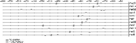
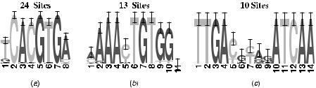
To illustrate this complexity, we look at an example in Saccharomyces cerevisiae. Figure 3.6 gives a schematic representation of the upstream sequences from 11 genes in S. cerevisiae that are regulated by the Cbfl–Met4p–Met28p complex and Met31p or Met32p in response to methionine (selected from [49]). The consensus, which is the dominant DNA pattern describing the motif, for these binding sites is given by TCACGTG for the Cbfl–Met4p–Met28p complex and AAAACTGTGG for Met31p or Met32p [49]. A logo representation [50] of the aligned instances of the two binding sites is shown in Figure 3.7. Such a logo represents the frequency of each nucleotide at each position, the relative size of the symbol represents the relative frequency of each base at this position, and the total height of the symbols represents the magnitude of the deviation from a uniform (noninformative) distribution. Figure 3.6 shows the locations of the two binding sites in the region 800 bp upstream of translation start. It is clear from this picture that there are several possible configurations of the two binding sites present in this data set. First it is important to note that motifs can occur on both strands. Transcription factors indeed bind directly on the double-stranded DNA and therefore motif detection software should take this fact into account. Second, sequences could have either zero, one, or multiple copies of a motif. This example gives an indication of the kind of data that come with a realistic biological data set. Palindromic motifs are, from a computational point of view, a special type of transcription factor binding site as it is a subsequence that is exactly the same as
FIGURE 3.6. Schematic representation of upstream region of set of coregulated genes. Several possible combinations of the two motifs are present: (1) motifs occur on both strands, (2) some sequences contain one or more copies of the two binding sites, or (3) some sequences do not contain a copy of a motif.
78 GENE REGULATION BIOINFORMATICS OF MICROARRAY DATA
FIGURE 3.7. Logo representation of three sets of known TFBSs in S.cerevisae and Salmonela typhimurium: (a) binding site of Cbfl–Met4p–Met28p; (b) binding site of Met31p or Met32p; (c) FNR binding site.
its own reverse complement. An example of a palindromic motif is found in the DNA binding protein that regulates genes involved in cellular respiration (FNR) motif of Figure 3.7c. The left part of consensus TTGA is the reverse complement of the right part, TCAA.
A second class of special motifs is comprised of gapped motifs or spaced dyads. Such a motif consists of two smaller conserved sites separated by a gap or spacer. The spacer occurs in the middle of the motif because the transcription factor binds as a dimer. This means that the transcription factor is made out of two subunits that have two separate contact points with the DNA sequence. The parts where the transcription factor binds to the DNA are conserved but are typically rather small (3 to 5 bp). These two contact points are separated by a nonconserved gap or spacer. This gap is mostly of fixed length but might be slightly variable. Figure 3.7c shows a logo representation of the FNR binding site in bacteria.
Currently another important research topic is the search for cooperatively binding factors [51]. When only one of the transcription factors binds, there is no or a low level of activation, but the presence of two or more transcription factors activates the transcription of a certain gene. If we translate this into the motif-finding problem, we could search for individual motifs and try to find, among the list of possible candidates, motifs that tend to occur together. Another possibility is to search for multiple motifs at the same time.
3.7.2. Oligonucleotide Frequency Analysis
The most intuitive approach to extract a consensus pattern for a binding site is a string-based approach, where typically overrepresentation is measured by exhaustive enumeration of all oligonucleotides. The observed number of occurrences of a given motif is compared to the expected number of occurrences. The expected number of occurrences and the statistical significance of a motif can be estimated in many ways. In this section we give an overview of the different methods.
3.7.2.1. Basic Enumerations Approach A basic version of the enumeration methods was implemented by van Helden et al. [49]. They presented a simple and fast method for the identification of DNA binding sites in the upstream regions from
3.7. SEARCHING FOR COMMON BINDING SITES OF COREGULATED GENES |
79 |
families of coregulated genes in S. cerevisiae. This method searches for short motifs of 5 to 6 bp long. First, for each oligonucleotide of a given length, we compute the expected frequency of the motif from all the noncoding, upstream regions in the genome of interest. Based on this frequency table, we compute the expected number of occurrences of a given oligonucleotide in a specific set of sequences. Next, the expected number of occurrences is compared to the actual, counted, number of occurrences in the data set. Finally, we compute a significance coefficient that takes into account the distinct number of oligonucleotides. A binomial statistic is appropriate in the case where there are nonoverlapping segments.
Van Helden et al. [15] have extended their method to find spaced dyads; these are motifs consisting of two small conserved boxes separated by a fixed spacer. The spacer can be different for distinct motifs and therefore the spacer is systematically varied between 0 and 16. The significance of this type of motif can be computed based on the combined score of the two conserved parts in the input data or based on the estimated complete dyad frequency from a background data set.
The greatest shortcoming of this method is that there are no variations allowed within an oligonucleotide. Tompa [52] addressed this problem when he proposed an exact method to find short motifs in DNA sequences. Tompa used a measure that differs from the one used by van Helden et al. to calculate the statistical significance of motif occurrences. First, for each k-mer s with an allowed number substitutions, the number of sequences in which s is found is calculated. Next, the probability ps of finding at least one occurrence of s in a sequence drawn from a random distribution is estimated. Finally, the associated z-score is computed as
Ns Nps zs ¼ p
Nps(1 ps)
The score zs gives a measure of how unlikely it is to have Ns occurrences of s given the background distribution. Tompa proposed an efficient algorithm to estimate ps from a set of background sequences based on a Markov chain.
3.7.2.2. Combinatorial Approaches Another important contribution in this field was made by Pevzner and Sze [53], who defined the motif finding in terms of a computationally challenging problem. The assumption from which they start is that motifs that can be considered as implanted are similar up to a given number of mutations c to a certain consensus sequence of length l. Keich and Pevzner [54] elaborated on the concept of (l, c)-motifs and defined a twilight zone where all motif finders would have a hard time finding the correct answers. In [53] a combinatorial approach is presented as WINNOWER and SP-STAR to solve this problem. WINNOWER is an iterative graph-based approach and uses substantial computational power. SP-STAR is an extension of this procedure by adding a heuristic to separate random signals from true signals. In [55] this method was further refined by introducing MULTIPROFILER, which incorporates two extensions: the utilization of the neighborhood of a word and the use of multipositional
80 GENE REGULATION BIOINFORMATICS OF MICROARRAY DATA
profiles. With MULTIPROFILER they managed to further push the performance of their motif-finding algorithms. Another combinatorial method was presented by Buhler and Tompa [56], who used random projections to define a set of instances that can be used to initialize EM for motif finding.
3.7.2.3. Suffix Trees Another interesting string-based approach is based on the representation of a set of sequences with a suffix tree [57, 58]. Vanet et al. [58] have used suffix trees to search for single motifs in whole bacterial genomes. Marsan and Sagot [57] later extended the method to search for combinations of motifs. The proposed configuration of a structured motif is a set of p motifs separated by a spacer that might be variable. The variability is limited to +2 bp around an average gap length. They also allow for variability within the binding site. The representation of upstream sequences as suffix trees resulted in an efficient implementation despite the large number of possible combinations.
3.7.3. Probabilistic Methods
While in the previous section a binding site was modeled as a set of strings, the following methods are all based on a representation of the motif model by a position weight matrix.
3.7.3.1. Probabilistic Model of Sequence Motifs In the simplest model, we have a set of DNA sequences where each sequence contains a single copy of the motif of fixed length. (For the sake of simplicity, we will consider here only models of DNA sequences, but the whole presentation applies directly to sequences of amino acids.) Except for the motif, a sequence is described as a sequence of inde-
pendent |
nucleotides generated according to a single discrete |
distribution |
u |
0 |
¼ |
||||||||
A |
, |
C |
, |
G |
, |
T |
T |
called the background model. The motif |
uW |
|
|
||
(q0 |
q0 |
q0 |
q0 ) |
|
itself is described |
||||||||
by what we call a position frequency matrix, which are W independent positions |
||||||
generated according to different discrete distributions qb: |
||||||
|
|
|
|
|
|
i |
|
|
qA |
qA |
. . . qA |
1 |
|
|
|
1 |
2 |
|
W |
|
|
0qC |
qC |
. . . |
qC |
||
uW |
B |
1 |
2 |
|
W |
C |
G |
G |
. . . |
G |
|||
|
¼ Bq1 |
q2 |
qW C |
|||
|
B |
|
|
|
|
C |
|
B |
T |
T |
. . . |
T |
C |
|
@ q1 |
q2 |
qW A |
|||
If we know the location sequence given the motif
ai of the motif in a sequence Si, the probability of this position, the motif matrix, and the background model is
ai 1 |
aiþW 1 |
|
|
L |
W q0Sij |
P(Sijai, uW , u0) ¼ Yj 1 q0Sij |
jYai |
qSjij |
aiþ1 j |
Yai |
|
¼ |
¼ |
|
|
¼ þ |
|
Wherever appropriate, we will pool the motif matrix and the background model into a single set of parameters u ¼ (u0, uW ). For a set of sequences, the probability of
3.7. SEARCHING FOR COMMON BINDING SITES OF COREGULATED GENES |
81 |
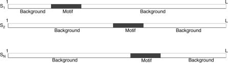
FIGURE 3.8. In this basic sequence model, each sequence contains one and only one copy of the motif. The first part of the sequence is generated according to the background model u0, then the motif is generated by the motif matrix uW , after which the rest of the sequence is again generated according to the background model.
the whole set S ¼ {S1, . . . , SN } given the alignment (i.e., the set of motif positions), the motif matrix, and the background model is
N |
|
P(S j A, u) ¼ Yi 1 P(Si j ai, u) |
(3:1) |
¼ |
|
The sequence model is illustrated in Figure 3.8. The idea of the EM algorithm for motif finding is to find simultaneously the motif matrix, the alignment position, and the background model that maximize the likelihood of the weights and alignments. Gibbs sampling for motif finding extends EM in a stochastic fashion by not looking for the maximum-likelihood configuration but generating candidate motif matrices and alignments according to their posterior probability given the sequences.
3.7.3.2. Expectation–Maximization One of the first implementation to find a matrix representation of a binding site was a greedy algorithm by Hertz et al. [59] to find the site with the highest information content (which is the entropy of the discrete probability distribution represented by the motif matrix). This algorithm was capable of identifying a common motif that is present once in every sequence. This algorithm has been substantially improved over the years [60]. In their latest implementation, CONSENSUS, Hertz and Stormo [60] have provided a framework to estimate the statistical significance of a given information content score based on large-deviation statistics.
Within the maximum-likelihood estimation framework, EM is the first choice of optimization algorithm. Expectation–maximization is a two-step iterative procedure for obtaining the maximum-likelihood parameter estimates for a model of observed data and missing values. In the expectation step, the expectation of the data and missing values is computed given the current set of model parameters. In the maximization step, the parameters that maximize the likelihood are computed. The algorithm is started with a set of initial parameters and iterates over the two described steps until the parameters have converged. Since EM is a
82 GENE REGULATION BIOINFORMATICS OF MICROARRAY DATA
gradient-ascent method, EM strongly depends on the initial conditions. Poor initial parameters may lead EM to converge to a local minimum.
For motif finding EM was introduced by Lawrence and Reilly [61] and was an extension of the greedy algorithm of Hertz et al. [59]. It was primarily intended for searching motifs in related proteins, but the method described could also be applied to DNA sequences. The basic model assumption is that each sequence contains exactly one copy of the motif, which might be reasonable in proteins but is too strict in DNA. The starting position of each motif instance is unknown and is considered as being a missing value from the data. If the motif positions are known, then the observed frequencies of the nucleotides at each position in the motif are the maximum-likelihood estimates of model parameters. To find the starting positions, each subsequence is scored with the current estimate of the motif model. These updated probabilities are used to reestimate the motif model. This procedure is repeated until convergence. Since assuming there is exactly one copy of the motif per sequence is not really biological sound, Bailey and Elkan proposed an advanced EM implementation for motif finding called MEME [62, 63]. Although MEME was also primarily intended to search for protein motifs, MEME can also be applied to DNA sequences.
To overcome the problem of initialization and getting stuck in local minima, MEME proposes to initialize the algorithm with a motif model based on a contiguous subsequence that gives the highest likelihood score. Therefore, each substring in the sequence set is used as a starting point for a one-step iteration of EM. Then the motif model with the highest likelihood is retained and used for further optimization steps until convergence. The corresponding motif positions are then masked and the procedure is repeated. Finally, Cardon and Stormo proposed an EM algorithm to search for gapped motifs [64]. However, while performing well for extended protein motifs, EM often suffers badly from local minima for short DNA motifs. An even more intelligent initialization procedure is the random-projections method of Buhler and Tompa [56].
3.7.3.3. Basic Algorithm for Gibbs Sampling for Motif Finding The probabilistic framework led to another important approach to solve the motiffinding problem. Gibbs sampling for motif finding was presented by Lawrence et al. [65] and was later described in more technical details by Liu et al. [66]. Gibbs sampling is a Markov chain Monte Carlo procedure that fits perfectly within the missing-data problem. While EM gives the maximum-likelihood estimates, the goal here is to model the posterior distribution and to generate data accordingly. Shortly said, the proposed algorithm is basically a collapsed Gibbs sampler which involves a Markov chain of the form:
Sample a(1tþ1)
Sample a(2tþ1)
Sample a(Ntþ1)
from p (a1 j a(2t), . . . , a(Nt), S).
from p (a2 j a(1tþ1), a(3t), . . . , a(Nt), S):
.
.
.
from p (aN j a(1tþ1), . . . , a(Ntþ1)1 , S).

3.7. SEARCHING FOR COMMON BINDING SITES OF COREGULATED GENES |
83 |
In words, the alignment position in sequence i is sampled according to a probability distribution dependent on the current set of alignment position in all other sequences. It can be shown that this Markov chain has the distribution p(A j S) as its equilibrium state [66]. The computation of these probability distributions involves the use of multinomial probability distributions (for the probability of the data based on the likelihood function presented in Section 3.7.3.1 and on the motif matrix and the background model) and Dirichlet probability distributions (for the probability of the parameters of the motif matrix). The derivation of the collapsed Gibbs sampler involves several properties of integrals of Dirichlet distributions and a number of approximations are used to speed up the algorithm further. To be concrete, we present here the resulting algorithm:
1.Input: A set of sequences S and the length W of the motif to search.
2.Compute the background model u0 from the nucleotide frequencies observed in S.
3.Initialize the alignment vector A ¼ fai j i ¼ 1, . . . , Ng uniformly at random.
4.For each sequence Sz, z ¼ 1, . . . , N:
(a) Create subsets S ¼ fSi j i = zg and A ¼ fai j i = zg. |
|
|
|
|
||||
(b) |
Compute uW |
from the segments indicated by A. |
|
|
|
|
|
|
e |
e |
|
|
|
þ |
|
||
(c) |
|
|
¼ |
. . . , Li |
W |
1) in Sz |
||
Assign to each possible alignment start (xz j, j e 1, |
|
|
||||||
a weight W(xz j) given by the probability that the corresponding segment is generated by the motif versus the background:
W(xz j) ¼ P(Sz j, . . . , Sz( jþW 1)juW )
P(Sz j, . . . , Sz( jþW 1)ju0)
YW qSz( jþk 1)
¼ z
qSz( jþk 1) k¼1 0
(d) Draw new alignment positions az according to the normalized probability
distribution W(xz j)= PLi Wþ1 W(xz j).
k¼1
5.Repeat step 4 until the Markov chain reaches stochastic convergence (fixed number of iterations).
6.Output: A motif matrix uW and an alignment A.
3.7.3.4. Extended Gibbs Sampling Methods Several groups proposed advanced methods to fine tune the Gibbs sampling algorithm for motif finding in DNA sequences. A first version of the Gibbs sampling algorithm that was especially tuned toward finding motif in DNA sequences is AlignACE [14], and this version was later refined [67]. This algorithm was the first reported to be used for the analysis of gene clusters. Several modifications were made in AlignACE with respect to the original Gibbs sampling algorithm. First, one motif at the time was retrieved and the positions were masked instead of simultaneous multiple motif searching.