

Genomics and Proteomics Engineering in Medicine and Biology - Metin Akay
.pdf134 IN SILICO RADIATION ONCOLOGY
mathematical model examining tumors as part of a dynamic society of interacting malignant and normal cells. Rizwan-Uddin and Saeed [16] presented predictions of a mathematical model of mass transfer in the development of a tumor, resulting in its eventual encapsulation and lobulation. Michelson and Leith [29] modeled the effect of the angiogenic signals of basic fibroblast growth factor (bFGF) and vascular endothelial growth factor (VEGF) on the adaptive tumor behavior.
Computer simulation models aim at three-dimensionally reconstructing a growing tumor based on the behavior of its constituent parts (either single cells or clusters of cells). Such models have been used in order to study, for example, the emergence of a spheroidal tumor in nutrient medium [30–38], the growth and behavior of a tumor in vivo [39–42], and the neovascularization (angiogenesis) process [31]. Duechting [31] developed a three-dimensional simulation model of tumor growth in vitro by combining systems analysis, control theory, and cellular automata. Wasserman and Acharya [39] developed a macroscopic tumor growth model mainly based on the mechanical properties of the tumor and the surrounding tissues. Kansal et al. [40, 41] proposed a three-dimensional cellular automaton model of brain tumor growth by using four parameters and introducing an adaptive grid lattice.
Experimental models of tumor response to radiation therapy primarily aim at determining the survival probability of the irradiated cells as a function of the absorbed dose (survival curves). The values of many other parameters of interest can also be estimated [43–45]. Mathematical models attempt to analytically describe the effect of ionizing radiation to tumor and normal tissue cells [5, 46–63]. Thames et al. [46] mathematically described the dissociation between acute and late radiation responses with changes in dose per fraction. Dale [51] extended the classical linear quadratic dose–effect relationship in order to examine the consequences of performing fractionated treatments for which there is insufficient time between fractions to allow complete damage repair. Fowler [53] reviewed the considerable progress achieved in fractionated radiotherapy due to the use of the linear quadratic model. Zaider and Minerbo [60] proposed a mathematical model of the progression of cells through the mitotic cycle under continuous low-dose-rate irradiation and applied it to studies of the effects of dose rate on HeLa cells. Jones and Dale [62] presented various modifications of the linear quadratic model that were used in order to optimize dose per fraction. Of special importance are the recent attempts to mathematically model the effect of specific genes (e.g., the p53 status) to the radiation response of tumors [64]. Haas-Kogan et al. [64] modeled two distinct cellular responses to irradiation, p53-independent apoptosis, and p53-dependent G1 arrest that characterize the radiation response of glioblastoma cells using the linear quadratic model. Mathematical modeling of chemotherapy and other treatment modalities that may be applied in parallel with radiation therapy has also been developed [65, 66].
Computer simulation models aim at three-dimensionally predicting and visualizing the response of a tumor [36, 67–86] or normal tissue [70] to various schemes of radiation therapy as a function of time. Nahum and Sanchez-Nieto [68] presented a computer model based on the concept of the tumor control probability (TCP)
5.3. PARADIGM OF FOUR-DIMENSIONAL SIMULATION |
135 |
and studied TCP as a function of the spatial dose distribution. Stamatakos et al. [71] developed a three-dimensional discrete radiation response model of an in vitro tumor spheroid and introduced high-performance computing and virtual reality techniques in order to visualize both the external surface and the internal structure of a dynamic tumor. Kocher et al. [76, 77] developed a simulation model of tumor response to radiosurgery (single-dose application) and studied the vascular effects.
Finally extensive work is being done on the combination of advanced visualization techniques, high-performance computing, and the World Wide Web capabilities in order to integrate and clinically apply the oncological simulation models [32–37, 79–81].
5.3. PARADIGM OF FOUR-DIMENSIONAL SIMULATION OF TUMOR GROWTH AND RESPONSE TO RADIATION THERAPY IN VIVO
5.3.1. Data Collection and Preprocessing
The imaging data [e.g., computed tomography (CT), magnetic resonance imaging (MRI), and positron emission tomography (PET)], the histopathologic (e.g., type of tumor) and genetic data (e.g., p53 status, if available) of the patient are appropriately collected. The distribution of the absorbed dose in the region of interest at the end of the physical treatment planning procedure is also acquired.
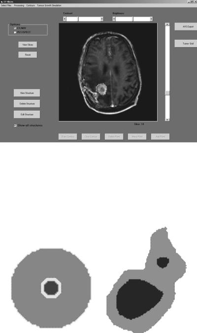
The imaging data are introduced into a dedicated preprocessing software tool. If imaging data from diverse modalities are available, appropriate image registration techniques are used [85]. The clinician delineates the tumor and other structures of interest by using the dedicated software tool (Fig. 5.1). Each structure consists of a number of contours defined in successive tomographic slices. Subsequently, the imaging data, including the definition of the structures of interest, are adequately preprocessed, so as to be converted into the appropriate form, which will constitute the input for the simulation software. Preprocessing includes interpolation procedures in case of anisotropic data: gray-level interpolation for the imaging data and, most importantly, shape-based interpolation for the structures of interest [85]. The interpolation procedure is applied to every structure of interest and the results are combined in an image that constitutes the input of the simulation software. In this final image each structure is represented by its characteristic gray level (Fig. 5.2).
5.3.2. Data Visualization
The output of the above procedure is introduced into the visualization package AVS (Advanced Visualization Systems)/Express 4.2, which performs the visualization of the region of interest. AVS/Express is also used for the visualization of the simulation results. AVS/Express offers highly interactive three-dimensional data visualization capabilities, which facilitate the analysis and interpretation of the
136 IN SILICO RADIATION ONCOLOGY
FIGURE 5.1. The interface of the dedicated software tool for the delineation of anatomical structures of interest and the preprocessing procedure of the imaging data.
modeling results. It provides predefined components (“modules”) for data acquisition and visualization with volumeor surface-rendering techniques. Predefined or user-defined modules can be combined to form complex “networks” of data manipulation. It offers modules for intersection of data in different cutting planes
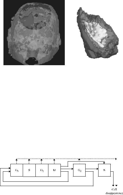
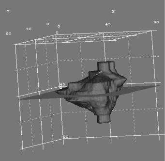
FIGURE 5.2. Indicative three-dimensional visualizations of the region of interest for a hypothetical tumor using AVS/Express 4.2.
5.3. PARADIGM OF FOUR-DIMENSIONAL SIMULATION |
137 |
FIGURE 5.3. Two-dimensional equatorial slices from two indicative three-dimensional input data for the simulation software. Each structure is represented by its characteristic gray-level.
and orientations. In addition, the use of coloring and transparency features facilitates the visual inspection of complex topologies. For surface-rendering techniques the final representation can be exported from the package in VRML 1.0 or 2.0 format and become available for study in a machine-independent and interoperable way for local or remote examination through a local network or the Internet. Indicative three-dimensional visualizations performed with AVS/Express are presented in Figure 5.3.
5.3.3. Biology of Solid Tumor In Vivo: Algorithmic Expression
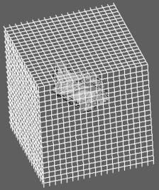
I. The cytokinetic model shown in Figure 5.4, based on the one introduced in [69, 70], is adopted. According to this model a tumor cell when cycling passes through the phases G1 (gap 1), S (DNA synthesis), G2 (gap 2), and M (mitosis). The corresponding maximum durations of these phases are designated TG1, TS,
FIGURE 5.4. Cytokinetic model of a tumor cell. Symbol explanation: G1: G1 phase, S: DNA synthesis phase, G2: G2 phase, G0: G0 phase, N: necrosis, A: apoptosis.
138 IN SILICO RADIATION ONCOLOGY
TG2, and TM. These durations, according to the literature, seem to follow the normal distribution. As a first approximation, we use the mean values of the duration of each cell cycle phase and neglect standard deviations.
After mitosis is completed, each one of the resulting cells reenters G1 if oxygen and nutrient supply in its current position are adequate. Otherwise, it enters the G0 resting phase in which, if oxygen and nutrient supply are inadequate, it can stay for a limited time (TG0). Subsequently it enters the necrotic phase, unless the local environment of the cell becomes adequate before the expiration of TG0. In the latter case the cell reenters G1. In addition, there is also a probability that each cell residing in any phase other than necrosis or apoptosis dies and disappears from the tumor due to spontaneous apoptosis (dashed line in Fig. 5.4).
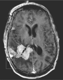
II. The description of the biological activity of the tumor is based on the introduction of the notion of the “geometric cell” (GC), the elementary cubic volume of a three-dimensional discretizing mesh covering the region of interest (Fig. 5.5). We assume that each GC of the mesh initially accommodates a number of biological cells (NBC). However, the maximum number of biological cells that can be accommodated in a GC is assumed to be NBCþNBC/2. Apparently NBC depends on the chosen size of the GC and determines the quantization error of the model. Biological cells are assumed to have a mass of 1029 gr [3]; a typical cell density is therefore 1026 cells/mm3. For example, in the case of a 1 1 1-mm GC, NBC would be equal to 106.
III. Each GC of the mesh belonging to the tumor is assumed to contain biological cells distributed in a number of equivalence classes (compartments), each one characterized by the phase in which its cells are found (within or out of the cell cycle, i.e., G1, S, G2, M, G0, necrosis, apoptosis).
FIGURE 5.5. A three-dimensional discretizing mesh covers the region of interest.
5.3. PARADIGM OF FOUR-DIMENSIONAL SIMULATION |
139 |
IV. All biological cells of a given class within a GC are assumed to be synchronized, which means that, at a particular instant, the time they have already spent in the cell cycle phase characterizing the class under consideration is the same. Biological cells belonging to the same class but in different GCs are not considered synchronized.
V. The distribution of the initial NBC of a GC in each phase class is estimated according to the position of the corresponding GC within the tumor, namely based on the estimated metabolic activity in the local area [e.g., through PET/SPECT (single photon emission computed tomography) or functional MRI]. The information derived from the imaging data directs the division of the tumor region into subregions [86]. The GCs belonging to the same subregion are considered to be of roughly the same metabolic activity. Hence, subregions considered “proliferating cell regions,” “resting-G0 cell regions,” or “dead cell regions” are defined. The determination of the relative fractions of proliferating, resting, and dead cells in each metabolic subregion depends on the histology of the tumor and on accumulated clinical experience. Such experience dictates, for example, that even a single alive clonogenic cell can repopulate a tumor mass).
VI. A “coloring criterion” must be formulated for the three-dimensional visualization of the simulation results. The coloring criterion “decides” on to which subregion a GC should be assigned at a specific instant. This rule is closely related to the definition of the subregions and to the current relative proportions of proliferating, resting, and dead cells within the GC. It also depends on the histopathological features of the tumor. As an example, in the case of glioblastoma multiforme tumors the following “98% coloring criterion” can be used:
For a GC of the discretizing mesh,
if the percentage of dead cells is lower than 98% then {if percentage of proliferating cells
>percentage of G0 cells then
{paint the GC with the proliferating cell region color}
else { paint the GC with the G0 cell region color}}
else
{paint the GC with the dead cell region color}
The main reason for intensifying the effect of the presence of proliferating and G0 cells in the above criterion is that even a single alive clonogenic tumor cell (either cycling or in G0) can lead to tumor recurrence.
VII. The initial distribution of the proliferating biological cells of a GC within each of the proliferating phases (G1, S, G2, M) is estimated using the duration of each cell cycle phase for the specific tumor.
5.3.4. Radiobiology of Solid Tumor in Vivo: Algorithmic Expression
The response of each cell to irradiation leading to absorbed dose D is described by the linear-quadratic (LQ) model, which is widely used in the pertinent literature
140 IN SILICO RADIATION ONCOLOGY
[3, 4, 69, 70]. According to this model, the survival probability S of a cell is given by the expression
S ¼ exp½ (aD þ bD2)& |
(5:1) |
where D is the absorbed dose and a, b parameters characterize the initial slope and the curvature, respectively, of the survival curve. Equation (5.1) can be used for fractionated radiotherapy provided that there exists a sufficient time interval between fractions for sublethal damage repair to be completed [3].
The radiosensitivity of cells varies considerably as they pass through the subsequent phases of the cell cycle, with the S phase regarded as the most resistant [3, 44]. Cells in any proliferating phase (G1, S, G2, and M) are more radiosensitive than hypoxic cells residing in G0. Furthermore, of particular notice is the fact that the parameters a and b of the LQ model constitute one possible way to incorporate the influence of genetic determinants, such as the p53 gene status (mutations or expression of p53 protein), into the simulation model [86].
5.3.5. Simulation Outline
Time is discretized and incremented. One hour has been adopted as the unit of time. In each time step the geometric mesh is scanned and the updated state of a given GC is determined as follows:
I.At the time instants that correspond to the delivery of a specific radiation dose D to the tumor, the number of cells killed in a particular GC is calculated based on the LQ model [Eq. (5.1)]. In a tumor growth simulation case, the dose D in Eq. (5.1) would be set to zero.
II.Lethally damaged cells following exposure to radiation undergo two mitotic divisions prior to death and disappearance from the tumor [4, p. 87].
III.At each time step the time registers of all GCs increase by 1 hour. All the necessary cell cycle phase transitions are computed.
IV. The possibilities of cell loss due to apoptosis and necrosis are computed by using the equations
CBR ¼ |
GF |
(5:2) |
|
|
|
||
TC |
|||
CLF ¼ |
CLR |
(5:3) |
|
|
|||
CBR |
|||
where CLF is the cell loss factor, CLR the cell loss rate, CBR the cell birth rate, GF the growth fraction, and TC the duration of the cell cycle. The total cell loss factor is assumed to be the sum of the cell loss factor due to necrosis and the cell loss factor due to apoptosis and to remain constant throughout the simulation. Future versions of the model will investigate the assumption of a time-varying CLF. Possible variations of the cell cycle duration throughout the simulation are also under investigation.
5.3. PARADIGM OF FOUR-DIMENSIONAL SIMULATION |
141 |
The simulation of tumor expansion or shrinkage is based on the following rules: If the actual number of alive and dead (but still morphologically existing) tumor cells contained within a given GC is reduced to less than NBC/2, then a procedure which attempts to “unload” the remaining biological cells in the neighboring GCs takes place aimed at emptying the current GC. The basic criterion of the unloading procedure states that the unloading process proceeds in such a way that the biological cell density of the entire lattice is as uniform and as close to “NBC per GC” as possible. Therefore, the unloaded cells are preferentially placed within the neighboring GCs having the maximum available free space. If two or more of the neighboring GCs possess the same amount of free space, then a random-number generator is used for the selection. If at the end of the unloading procedure the given GC becomes empty, it disappears from the tumor. An appropriate shift of a chain of GCs, intended to fill the “vacuum,” leads to differential tumor shrinkage. This can happen, for example, after a number of cells are killed due to irradiation.
On the other hand, if the number of alive and dead cells within a given GC exceeds NBCþNBC/2, then a similar procedure attempting to unload the excess cells in the surrounding GCs takes place. If the unloading procedure fails to reduce the number of cells to less than NBCþNBC/2, then a new GC emerges. Its position relative to the “mother” GC is determined using a random-number generator. An appropriate shifting of a chain of adjacent GCs leads to a differential expansion of the tumor. The “newborn” GC initially contains the excess number of biological cells, which are distributed in the various phase classes proportionally to the distribution in the mother GC. The impact of the definition of the upper and lower thresholds, which in the present case have been set to NBC þ NBC/2 and NBC2NBC/2, respectively, on the uniformity of the distribution of the biological cells throughout the lattice is under investigation.
The differential tumor expansion and shrinkage algorithms are based on the use of random-number generators in conjunction with adequately formed morphological rules. These rules aim at tumor shrinkage or expansion conformal to the initial shape of the tumor. This is a logical assumption if the pressure in the normal tissues surrounding the tumor region is assumed to be uniform and the tumor is not in contact with practically undeformable tissues such as the bone.
More specifically, in the case of selection of shrinkage direction, the outermost tumor GC is detected along each one of six possible directions of shrinkage (Cartesian coordinate system XYZ centered at the current GC, each axis defining two possible directions of movement). Its “six-neighbor” GCs belonging to the tumor (NGCT) are counted. The direction corresponding to the maximum NGCT is finally selected out of the six possible directions as the direction along which the shifting of the GCs will take place (shifting direction). If more than one shifting direction has the same maximum NGCT, then the selection is based on the use of a random-number generator. A similar, though inverse, morphological-mechanical rule can be applied in the case of tumor expansion. An alternative algorithm, which will be used in future versions of the simulation model, performs shrinkage and expansion along a line of random angle. In this way, artifacts attributed to the movement of GCs along the axes of the Cartesian coordinate system will be avoided.
142 IN SILICO RADIATION ONCOLOGY
The need for the formulation of the above morphological rules for tumor shrinkage and expansion has arisen from the inspection of the macroscopic results of the simulation algorithms. A completely random selection of one out of the six possible shifting directions results in a premature extensive fragmentation of the tumor region in case of radiotherapy, which is usually incompatible with clinical experience. The general trend is a conformal shrinkage of most solid tumors (Fig. 1.4 in [4]).
The mechanical properties of the surrounding normal tissue are considered uniform around the tumor, with the exception of an absolute lack of deformability of the bone. As a first approximation, immunological reactions, invasion, and formation of metastases have been ignored.
5.3.6. Parametric Testing of Simulation Model: Case of Glioblastoma Multiforme Irradiated by Various Fractionation Schemes
A case of a glioblastoma multiforme (GBM) tumor recently irradiated has been selected. A specialized doctor has delineated the clinical boundary of the tumor and its necrotic area based on the corresponding MRI and PET data after irradiation (Fig. 5.6) (hysteron proteron for validation reasons). A three-dimensional mesh quantizing the anatomical region of interest has been considered. The dimensions of each GC are 1 1 1 mm. Such a volume contains roughly 106 biological cells (NBC ¼ 106). Figure 5.7 depicts a three-dimensional visualization of the tumor before the beginning of radiotherapy treatment.
FIGURE 5.6. An MRI slice depicting a glioblastoma multiforme brain tumor recently irradiated. Both the clinical volume of the tumor and its central necrotic area have been delineated.
5.3. PARADIGM OF FOUR-DIMENSIONAL SIMULATION |
143 |
FIGURE 5.7. Three-dimensional visualization of the tumor before the beginning of the irradiation. Volume rendering produced with AVS/Express 4.2.
As no information about the metabolic activity (and therefore the density of the tumor neovasculature) prior to irradiation was available (e.g., through PET or functional MRI) for the particular case considered, the growth support criterion applied so far was the minimization of the distance from the outer surface of the tumor. This implies that biological cells residing in the outer layer of the tumor (“proliferating cell layer”) can be adequately oxygenated and fed whereas the inner part of the tumor (“dead-cell layer”) lacks efficient neovasculature and therefore oxygenation and nourishment. An intermediate layer containing a significant amount of G0 cells has also been assumed (“G0 cell layer”) . Obviously, the above layered structure may not be the case in a large number of tumors. If, for example, the metabolic imaging data (e.g., PET, SPECT, functional MRI) prior to irradiation suggest that the metabolic activity of the tumor is rather uniform throughout its volume, the growth support criterion would become rather uniform too. For the specific type of tumor all nonclonogenic cells are considered to be necrotic (sterile cells are not taken into account). This is a logical first approximation, since GBM is generally considered a poorly differentiated type of tumor. A typical clonogenic cell density is 107 to 108 cells/cm3 (104 to 105 cells/mm3) [62, 68]. We assume a clonogenic cell density of 2 104 cells/mm3 in the proliferating cell layer (a 6-mm-thick layer from the outer boundary of the tumor), 104 cells/mm3 in the G0 cell layer (a 1-mm-thick