X-Ray Methods for the Characterization of Nanoparticles

164 7 X-Ray Methods for the Characterization of Nanoparticles

make this chapter easier reading for those without an extensive background in physics, this is done in quite a perceptual way, starting from what is measured and showing what information can be derived from it based on selected (partly idealized) examples. For a more rigorous formal description of these processes, which leads to the formulas and statements used in the following sections and any in-depth approach, the interested reader is referred to the Appendix of this chapter. After this introduction to the potential of the respective techniques, their specific application to nanoparticles is discussed from a critical perspective in relation to three examples, which are intended to show not only the strengths but also the weaknesses of the respective methods.

7.2

X-Ray Diffraction: Getting to Know the Arrangement of Atoms

In x-ray diffraction, elastic scattering processes are observed, i.e., the coupled values photon wavelength and photon energy remain constant, and so does the state of the scattering system. At the same time, the scattered x-rays stay coherent. Only the direction of propagation is changed, which is often described using the scattering vector, defined by the relation

(see also Fig. 7.1, and also the complete list of variables given at the end of this chapter). Consequently, what needs to be determined in an x-ray diffraction experiment is the probability of finding a scattered photon in a given solid angle element.

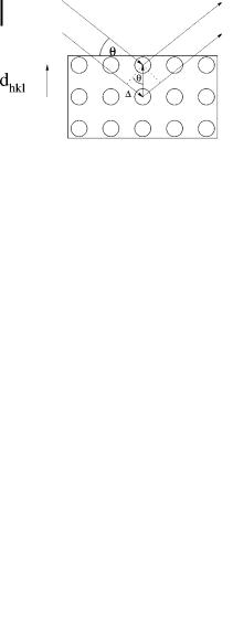
Figure 7.1. Derivation of the Bragg condition for x-ray diffraction.

The most elementary way to arrive at a statement of under what conditions intensity can be found in a given solid angle element can be derived from Fig. 7.1: in order to obtain a strong signal under a Bragg angle HB measured relative to a given lattice plane, contributions of scattering events which occur in neighboring lattice planes must be in phase, i.e., the difference in the optical path length must be given by

7.2 X-Ray Diffraction: Getting to Know the Arrangement of Atoms 165

Table 7.1. Different approaches for the measurement of x-ray diffraction data.

which is exactly the Bragg condition. It should be stressed that this condition is necessary but not sufficient: it selects only the discrete angles under which diffraction may be observed and does not provide the angles under which it will be observed, because it is related only to the structural scattering factor discussed in the Appendix (Section A.3). It should also be noted that one can conclude from this formula that the smaller the wavelength of the photon, and therefore the higher its energy, the better the resolving power of the method, because more lattice planes/combinations of Miller indices hkl can be probed. Of course, in order to obtain a complete description of the structural arrangement, more than one reflection is needed. There are several experimental approaches to achieving this. The first distinction is whether one offers a broad distribution of wavelengths [e.g., the white light obtained from a synchrotron radiation (SR) source] or uses a monochromatic source (e.g., monochromatic SR beam or a characteristic line of an x-ray tube). The second distinction is whether a sufficiently large single crystal can be produced or not. The possible

Figure 7.2. (a) Simulated Cu Ka XRD spectra of hcp (red) and fcc (black) Co. (b) Simulated Cu Ka XRD spectra of NaCl (red) and KCl (black).

166 7 X-Ray Methods for the Characterization of Nanoparticles

approaches for obtaining a complete set of XRD data which emerge from the combination of these two criteria are summarized in Tab. 7.1.

Evidently, nanoparticles are not very good single crystals; therefore measurements in Laue geometry are not possible and one needs to perform powder diffraction experiments. Detailed information on common setups and instrumentation for the methods mentioned above can be found in the literature, e.g., Ref. [1] for laboratory source-based experiments, Ref. [2] for SR-based experiments on single crystals, and Ref. [3] for SR-based powder diffraction experiments.

What can one learn from a powder x-ray diffraction spectrum, as displayed in Fig. 7.2? In the description presented so far, we have just correlated a geometric arrangement of scattering centers and an angle under which the scattered photon is found one correlates [A) the geometric arrangement of scattering centers] and [B) the angle under which the scattered photon is found] to each other. Even though this information is not all that can be gained in an XRD experiment, it is of considerable use. The reason for this is that the shape and size of the unit cell of a given crystal can be deduced from the angular positions of the diffraction lines, as evident for the comparison of simulated hcp and “face centered cubic” Co spectra shown in Fig. 7.2(a) and discussed in more detail e.g., in Ref. [1]. Based on the combination of Bragg’s law and the properties of the seven systems into which all crystals can be classified (cubic, tetragonal, orthorhombic, trigonal/rhombohedral, hexagonal, monoclinic, and triclinic), one obtains equations which allow indexing of the observed XRD peaks. For example, in a cubic system with lattice constant a, dhkl is given by

a

dhkl ¼ p (3) h2 þk2 þl2

The next step consists in the determination of the number of atoms per unit cell. This is easily obtained, as the volume of the unit cell is readily calculated based on the parameters determined so far, and usually the density of a given material is obtained easily and its chemical composition can be determined. Therefore, the weight of a unit cell can be determined and must correspond to an integer number of atoms of the respective types.

What remains to be done is the assignment of the atoms to the respective positions, which can be done using the information contained in the intensity of the respective scattering peaks (after correcting for additional effects which can influence this intensity, such as multiplicity, Lorentz, absorption, and temperature factors). A vivid example of this is provided in Fig. 7.2(b), which shows the simulated Cu Ka XRD spectra of NaCl and KCl, which belong to the same space group but have a different lattice distance. Due to the latter, the angular positions of the respective Bragg peaks are shifted, but it is easy to identify the structures which correspond to each other. However, there are notable differences in absolute and relative

7.2 X-Ray Diffraction: Getting to Know the Arrangement of Atoms 167

intensities: in general, the intensity is consistently higher for the KCl spectrum. This is due to the higher scattering power of K relative to Na, and from the observation of how much this difference changes the intensity of a given peak can be derived which types of atoms are located at the lattice sites which contribute to a given Bragg peak. In fact, this is the key problem of structural determination for a new class of material using XRD, because a stepwise solution to the problem does not exist. Whereas in some cases comparison of the relative intensities of the respective Bragg reflexes and/or the information on chemical composition can suggest some possible site occupations, more often than not a brute force approach has to be used, distributing the atoms on the possible crystallographic sites and calculating the diffraction pattern which corresponds to this elementary cell of given symmetry and size. Naturally, the number of feasible combinations scales with the size of the elementary and the number of atoms which it contains. This is also the reason why CPU power is a critical factor in protein crystallography (cf. Ref. [2]), where elementary cells tend to be huge and contain several hundreds to thousands of atoms.

Note also that in the entire above description we have implicitly assumed that one is really dealing with a signal originating from a single phase of matter. Imagine the task of indexing reflexes in a mixture of several compounds in the right way! Also, especially with respect to the application of the method to nanoparticles, (see examples in Section 7.1.5 and theoretical background in A.2), the resolving power of XRD is strongly correlated to the number of elementary cells in the crystallites which are investigated, because this exerts direct influence on the width of the diffraction lines. Broadening of the Bragg reflexions is typically observed for particles with diameters below 100 nm. This is due to the fact that strictly speaking the Bragg condition is just a limiting case, as seen in the more detailed analysis of elastic scattering processes discussed in A.2. Of course, it is possible to attempt to make use of the broadening , e.g., by applying the Scherrer formula

in order to determine the particle size. However, upon comparison of as-determined particles sizes and the ones observed directly, e.g., from high-resolution transmission electron microscopy (HRTEM) pictures, XRD tends to yield considerably larger particle sizes (cf., e.g., Ref. [4]).

With respect to these complications, it is fortunate that today the application of XRD rarely involves the actual determination of a completely new crystal structure. Instead, in most cases the XRD data obtained on a given compound are compared to the huge crystal structure databases like the International Crystal Structure Database (ICSD) available today, which has opened up the possibility of fitting a given XRD spectrum by a method known as the Rietveld method [5, 6]. In this approach, a structural model is refined to reproduce the experimental data, using intensity correction parameters, lattice parameters, and possible zero shifts of the detection system, the lineshape, crystal structure parameters, and the background. To achieve this fit, after indexing the observed diffraction patterns and determination of possible space groups, lattice parameters are refined. Already during this process, the presence of several phases

168 7 X-Ray Methods for the Characterization of Nanoparticles

1000

900

800

700

600

500

400

300

200

0

2 Theta/º

Figure 7.3. Measured XRD data of a Co50Fe50 nanoparticle produced by laser ablation. (Figure kindly provided by K. Moras, Technische Universit t Clausthal, based on measurements by Dr. R. Kleeberg, Technische Universit t Freiberg)

Table 7.2. Results of Rietveld analysis for a 10-nm Fe50Co50 nanoparticle. Quartz and wuestite are artifacts due to sample preparation.

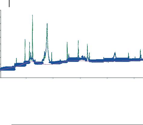
can be identified. The rough structure obtained from this processing step is then compared to isomorphous compounds or compounds which feature a similar structure contained in a database in order to obtain candidates for lattice site occupation. If the corresponding calculated diffraction pattern is similar to the observed one, refinement of the above parameters is performed. However, it should be noted that whereas obtaining a dissatisfying fit quality leads automatically to a change in the structural model, even a well-fitting result needs to be checked carefully for its chemical and physical relevance. Extreme values of the thermal displacement factor for a given site may indicate that it is occupied incorrectly; further parameters to be checked are bond lengths and bond angles, coordination numbers, and Madelung energies. An example of the result of a Rietveld refinement on a real XRD spectrum

7.3 Small-Angle X-Ray Scattering: Learning About Particle Shape and Morphology 169

of a 10-nm nanoparticle with nominal composition Fe50Co50 is shown in Fig. 7.3 and summarized in Tab. 7.2. Bearing in mind the considerable broadening of the peaks and a notable, angle-dependent background contribution, it is evident that in such a system much of the clarity intrinsic to XRD on macroscopic systems is lost.

7.3

Small-Angle X-Ray Scattering: Learning About Particle Shape and Morphology

As in the XRD measurements discussed above, in a SAXS experiment elastic scattering processes into a given solid angle element are observed, but this time – as indicated by the name of the technique – the detector covers only small scattering angles (typically less than 1 ). Looking at the Bragg condition discussed above, it is immediately clear that in a perfect, extended crystal this is a futile attempt – there is no scattering in that direction. However, this observation is based on destructive interference, which can only occur for a particle of dimension D if for a given x-ray another ray with a path difference k/2 also exists, i.e., if

This formula indicates that for a given x-ray wavelength the determination of the threshold angle under which scattering can just be observed yields information on the dimension of the particle. To illustrate this, let us assume that we are dealing with homogenous particles of uniform size and shape which are embedded in a homogenous matrix. In this case, it is possible to reduce the more complex description relying on local electron densities as described in appendix A.3, but also in

where the last term represents a factor which is dependent on the particle shape and is the Fourier transform of a radial distribution function of the scattering centers in a given atom, the so-called “form factor” S1. Some form factors for frequently encountered shapes are listed in Tab. 7.3. Note that in the above formula only the square of the scattering contrast is relevant, which means that the SAXS signal of a particle of chemical composition A in a matrix composed of B and particle B in matrix A are equivalent. However, this is only true if anomalous scattering effects [i.e., terms beyond the first term in Eq. (A6)] are negligible. The variation of scattering amplitudes, which is induced, e.g., in the vicinity of absorption edges of a given element due to these effects, can be used easily to separate the scattering contributions from matrix and particle, by subtraction of spectra which have been measured at two different photon energies, which cancels the contributions of the matrix, which stay constant, but not the varying ones of the particle. This approach is called ASAXS.

7.3 Small-Angle X-Ray Scattering: Learning About Particle Shape and Morphology 171

Also, it is possible to develop the form factor S1 in terms of powers of qr, which leads to the Guinier approximation

In this approximation, a fit of the scattering behavior for small values of qr yields the Guinier radius Rg, which is defined by the relation

and be considered as an analogon of the radius of gyration known from mechanics. A general expression for this radius as a function of particle radius R is

s

where the parameters n1, n2, and C are given for selected particle shapes in Tab. 7.3. Therefore, starting from the most simple assumption, i.e., particles A are present in matrix B, from the general shape of the scattering curve it is possible to gather information on particle shape and particle surface by fitting the high q and low q area, respectively, of the scattering curve. In combination with the integral scattering intensity Q0, which is obtained by integration of Eq. (7) over the entire q-space and

correlated to the total volume contribution constant C of phase A via the relation:

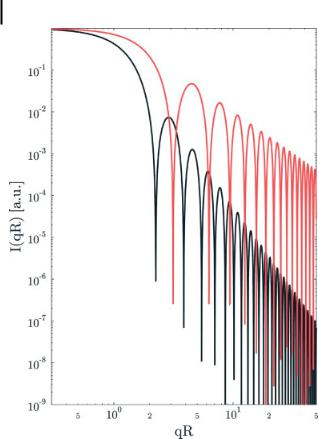
Using this set of relations, a good starting point for development of a structural model can be defined. As an example, consider the ideal calculated scattering crosssections for a sphere and a disk, respectively, which are displayed in Fig. 7.4.

Evidently, the asymptotic behavior of the scattered intensity is characteristic for a given shape and limits applicable structural models. Summing up, the SAXS method is an extremely sensitive tool for extracting information on particle morphology. However, it has a drawback which is due to its strength: as the exact extracted intensity distribution is sensitive to a large number of factors, in general the structural refinement which is applied to it is based on a number of implicit assumptions on the nature of the particle. For example, an inherent assumption which is frequently made is that the particle size distribution should follow a lognormal distribution, which is then fit to the data. Therefore, for the successful extraction of particle composition and shape, often additional information or confirmation is needed in order to arrive at a unique structural solution. Further details on SAXS and instrumentation for suitable experimental setups are found in, e.g., Refs. [7–9].

172 7 X-Ray Methods for the Characterization of Nanoparticles

Figure 7.4. Scattering cross-section signal for sphere (black) and spherical shell (red) of radius R. Note the asymptotic behavior for large qR, from which direct statements on the particle shape can be derived.

7.4

X-Ray Absorption: Exploring Chemical Composition and Local Structure

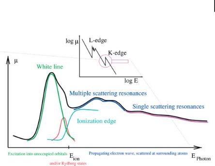
X-ray absorption spectroscopy (XAS) experiments measure the dependence of the cross-section of the absorption process (i.e., the probability that it occurs) on the energy of the incoming photon. The insert in Fig. 7.5 displays the trend which is observed upon a variation of photon energy in big steps over an extended energy range. It reflects the electronic structure of the corresponding element: steps in the cross-section occur whenever the photon energy is sufficiently high to excite electrons from a deeper core level; at the highest energy from the 1s level, proceeding with decreasing photon energy to 2s, 2p1/2 and 2p3/2, and so on. However, there are bound unoccupied states, and thus even at energies slightly lower than the ionization threshold it should be possible to excite the electrons into bound unoccupied

7.4 X-Ray Absorption: Exploring Chemical Composition and Local Structure 173

states. In fact, scanning an absorption edge in steps of the order of 1 eV, one observes a spectrum as shown in Fig. 7.5.

Figure 7.5. X-ray absorption fine structures and their (dominant) cause.

The absorption edge, i.e., the onset of the increase in the absorption cross-section, lies in fact at lower energies than the ionization energy. Also, at energies higher than the ionization threshold oscillatory structures are observed. This observation can be explained in a simple model if one recalls that in fact the photoelectron propagating through matter can be treated as a spherical wave, whose wavenumber k is connected with the energy of the incoming photon E and the ionization energy E0

where me represents the electron mass and h the normalized Planck’s constant. This photoelectron wave propagates through an environment in which it undergoes electron–electron scattering processes. Due to interference of outgoing and scattered wave, what one observes is an interference pattern, as schematically displayed in Fig. 7.6(a) for the case of constructive interference. On the other hand, varying the energy of the incoming photon varies the wavelength of the photoelectron; the interference pattern changes towards destructive interference, as shown in Fig. 7.6(b), and back to constructive interference. This explains the modulations observed in the absorption cross-section. Furthermore, the scattering probability is a function of the energy of the photoelectron, consequently in the energy region just above the absorption edge multiple scattering will be possible, and a large number of strong interference terms appear in the spectrum. These strong spectral features are called shape resonances. For histor-

174 7 X-Ray Methods for the Characterization of Nanoparticles

ical reasons, the first two regions are known as x-ray absorption near edge structure (XANES) – also called near edge x-ray absorption fine structure (NEXAFS), the latter is known as the extended x-ray absorption fine structure (EXAFS).

Figure 7.6. Constructive (a) and destructive (b) interference of outgoing and backscattered electron wave. Recall that the wavelength of the photoelectron depends on the energy of the incoming photon.

Even this rough understanding of the fine structure which appears in the absorption spectrum allows an estimation of the information one can obtain using this method: at the absorption edge, the unoccupied valence states are probed by the absorption process. But chemistry modifies the valence state/electronic structure of the elements, so one obtains information on the chemical environment of the absorber atom in the sample, which can be selected by choosing the excitation energy. At the same time, the interference pattern is characteristic for a given arrangement of the atoms which surround the absorbing atom and allows the extraction of information on its local coordination geometry without any need for long range order.

For the XANES structures, these effects are demonstrated at the Co K-edge in Fig. 7.7. In Fig. 7.7(a), a number of Co K-edge XANES spectra of compounds with varying formal oxidation state are displayed. Clearly, the onset of the structures shifts to higher energies with higher formal oxidation state. This is a rather systematic effect called “chemical shift.” Also, intensities of absorption in the white line range vary notably, which is correlated to the density of (atom-projected) unoccupied states, which tends to be higher for higher formal oxidation states. In Fig. 7.7(b), calculated spectra of metallic Co phases are displayed. Clearly, these spectra do not show chemical shift, but they do still show changes in their electronic structure. Perhaps even more interesting is the comparison of the shape resonances in the energy region between 7760 and 7840 eV (on the energy scale of the calculation), because it demonstrates clearly the localized point of view of the method: Co–Co distances in hcp and fcc Co are quite similar to each other, as demonstrated in Tab. 7.4. As a consequence, the shape resonances are also quite similar to each other, indicating that in fact the local environment and not long range order exert the dominating influence on the spectra.

1767 X-Ray Methods for the Characterization of Nanoparticles

Table 7.4. Local first and second shell coordination geometry of real and hypothetical metallic Co phases.

This is also the reason why a fingerprint approach to the interpretation of XANES spectra is so successful. Simple comparison with known reference substances allows, for example, the direct extraction of information on electronic structure, e.g., formal valency, and local coordination geometry in most cases. Due to their sensitivity to the local environment, XANES spectra are additive, i.e., a spectrum of a mixture of compounds A and B can be composed by weighted addition of the spectra of the pure reference compounds. This approach is called “quantitative analysis,” discussed in more detail, e.g., in Ref. [10] and frequently used for speciation purposes.

Fitting a structural model to the interference pattern in an x-ray absorption spectrum is possible in the EXAFS region using a path-by-path approach that allows for the analytic extraction of structural parameters. The general idea of this approach is given in Fig. 7.7; a more detailed description of the process is given in Section A.4.

Further information on XAS and XAS instrumentation is found in several books, reviews on the method, and conference proceedings [11–14].

7.5

Applications

A huge selection of nanoparticle characterizations using the above x-ray techniques exclusively or in combination is available in the literature. Rather than discussing these examples in detail, I will discuss a selection of three cases which illustrate the respective strengths and problems of the techniques introduced above.

7.5.1

Co Nanoparticles with Varying Protection Shells

A lot of scientific interest has recently been focused on Co nanoparticles. The main reason for this lies in their favorable magnetic properties, which in turn open a broad field of possible applications. They can be used, for example, in ultra-high- density magnetic media, magnetoresistive devices, ferrofluids, and magnetic refrigeration systems. Also, with respect to the topic of this book, biomedical applications should be mentioned, such as contrast enhancement in magnetic resonance imaging, magnetic carriers for drug targeting, and catalysis [15–17].

Numerous techniques have been used in studies [18–21] on this class of nanoparticles, including XAS. In fact, Fig. 7.8 displays the Co K-edge XANES spectra of a

7.5 Applications 179

pre-edge structure of these spectra grows with the particle size, whereas the maximum absorption decreases. In general, resemblance to the hcp Co spectrum increases, as the observed changes in intensity occur at those energy positions where spectral features in the Co foil spectrum are located, but even the spectrum of the largest particles differs from pure hcp Co. This suggests that addition of the hcp Co spectrum and the smallest nanoparticle spectrum might reproduce the spectra of both the 11-nm and the 8-nm particles by linear superposition of the spectra of the smallest particle, whose diameter is 5.5 nm, and that of hcp Co as shown also in Fig. 7.9. From this fit, an additional hcp content of about 40% for the 11-nm particle and of about 18.5% for the 8-nm particle can be derived. The error range for these numbers can be estimated to be –5%. As TEM pictures show homogenous particles and no indication of additional phases, this observation can be interpreted assuming a core–shell type structure of the particles. Assuming spherical particles and that the pre-edge intensity present in the spectrum of the smallest particle can be directly correlated to the amount of metallic Co present in this particle (40%), it is possible to extract the thickness of the respective cores and shells for the particles from the hcp Co contributions. The determined contribution of this phase is then given by the quotient of the cube of the core radius rc and the cube of the total radius rt. Performing this calculation, one obtains a core radius of 4.75 nm for the particles of 11 nm diameter, a core radius of 3.15 nm for the particles of 8 nm diameter, and a core radius of 2 nm for the 5.5-nm particles. All values indicate that the shell thickness is always 0.8 nm, which in turn enhances the plausibility of the assumptions. Further support for the formation of a core–shell system stems from an aging experiment discussed in Ref. [26].

Still, the nature of the shell needs to be identified. Likely candidates for the shell would be a Co oxide, such as CoO or Co2O3. (cf. Fig. 7.9). Due to the high similarity between the spectral features of the latter spectrum and the observed white line of the smallest nanoparticle, this may seem to be a good candidate, but the reproduction of the XANES spectra of the smallest particle by a linear superposition of the spectra of hcp Co and the corresponding oxide fails completely. In addition, the assumption of Co2O3 as being the compound forming the shell faces the problem that prolonged exposure to air converts the particles to CoO, and annealing removes the shell, which is inconsistent with assuming any type of oxide for the shell, because of the high stability of oxides. However, the comparison of the spectrum of the smallest particle to the ones of the different Co(II) reference spectra indicates clearly that, under the assumption that the shell material dominates the constituents of the smallest particle, this material must contain Co(III). Keeping in mind also that the shell is destroyed completely at very low temperatures of ~210 C [26], more likely candidates for the shell are Co(III) complexes such as Co[(NH3)6]Br3 and Co[(NR3)6]Br3. The formation of these complexes and also the observed core– shell structure of the particles seem to be “typical” of CTAB as none of these effects have been reported for Co nanoparticles stabilized with other surfactants, whereas, interestingly, a similar result has been obtained in a recent XAS study on CTAB-sta- bilized CeO2 nanoparticles, which were reported to possess a Ce3+ shell [27].

1807 X-Ray Methods for the Characterization of Nanoparticles

7.5.2

PdxPty Nanoparticles

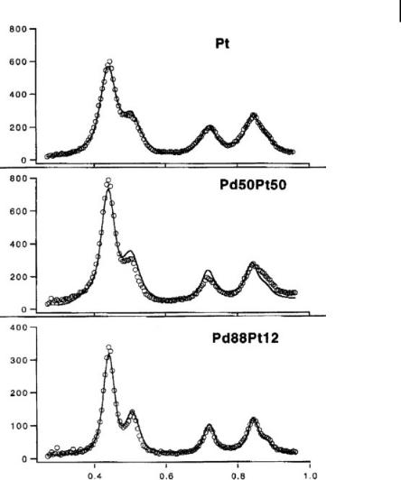
While the samples discussed in this example are of minor importance for biomedical application, they are of tremendous significance for applications in catalysis, where binary and ternary Pt catalysts on the nanoscale play a crucial role and are the subject of numerous investigations [28–31]. A key question in this context is how the arrangement of atoms in such a nanoparticle will actually look: will there be an ordered alloy, a statistical distribution of neighbors, a core–shell system, or some internal segregation and grain formation? At the same time, this system is especially suited for discussion in this chapter, as it can be used nicely to characterize the problems often encountered when applying XRD techniques to binary metallic systems such as alloys and intermetallic compounds. As an example of these problems, have a look at the XRD spectra of three PdxPt100-x nanoparticles with particle sizes of about 3.2–0.4 nm (as determined by TEM) shown in Fig. 7.10. Evidently, the differences between the obtained XRD spectra are rather small, and therefore a detailed determination of corresponding structures is hardly possible using this approach. A Rietveld analysis of this system will of course yield different results for different particles, but taking into account the lack of clarity of these structures, the statements derived from it may seem as questionable as the ability of XRD to distinguish between the different types of structures mentioned above. In fact, this is easily understood: the two metals under consideration are perfectly miscible in each concentration; both crystallize in fcc structure with lattice constants which vary by only 0.03 &.

Still, the EXAFS data from the same materials lead to different interference signals and consequently (non-phase-corrected) radial distribution functions which show clear differences even under mere visual inspection, as shown in Fig. 7.11 for the two bimetallic types of nanoparticles. The results of the analysis are summarized in Tab. 7.5. As a general trend, a lattice contraction is observed, which is stronger in the bimetallic particles. This is a trend which is frequently encountered in the analysis of small nanoparticles in general and was especially reported for a number of similar bimetallic particles by several authors (Refs. [25, 28–31] and references therein). Another striking effect is the significant reduction of the determined coordination numbers. This, too, is frequently encountered in nanoparticle systems. Partly, this meets the expectations, because a considerable share of the constituent atoms of a nanoparticle is located at its surface and thus not fully coordinated; but the observed reduction cannot be fully explained by this argument. However, such estimates assume the presence of perfect particles and perfect particle surfaces, which might not be an adequate description of the situation considering, e.g., the theoretical results obtained in Ref. [32]. A similar approach to the explanation of drastically reduced coordination numbers obtained when analyzing Fe nanoparticles has been suggested, e.g., by Di Cicco et al. [33, 34]. Another problem one does encounter is that Debye–Waller factors may no longer be described correctly, which are connected in the standard analysis to the gaussian pair distribution function which is the basis for the inclusion of the effective pair distribution in the

7.5 Applications 181

Figure 7.10. X-ray diffraction data of PdxPt100-x nanoparticles. Note the extreme similarity between the data sets! (From Ref. [54].)

Debye–Waller factor. This assumption is clearly questionable in the case of nanoparticles. Rather, one might encounter a bond-length distribution which is shaped like an asymmetric double-well potential and thus far from the gaussian ideal. As a matter of fact, Babanov et al. [35] have performed a more general EXAFS analysis on Co nanoparticles and reached the conclusion that in a boundary layer of the particles a four-fold coordination might be observed. Apart from an asymmetric static radial distribution function discussed in Ref. [35], anharmonic Co–Co vibrations could lead to a dynamic asymmetry in this function, as discussed in detail in Ref. [36].

182 7 X-Ray Methods for the Characterization of Nanoparticles

Figure 7.11. EXAFS analysis of PdxPt100-x nanoparticles. (a, c) v(k) function and fit; (b, d) modified Fourier transform and fit. (From Ref. [54].)

Even though the absolute coordination of the absorbing atoms is frequently underestimated, the relative coordination numbers can yield important information on the arrangement of the various types of atoms. As evident from Tab. 7.5, the relative coordination numbers of a Pt absorber meet the purely statistical prediction reasonably well for the Pd-rich particles, whereas the contribution of Pt neighbors is

7.5 Applications 183

higher than such a model would predict. This result can be explained by a nonstatistical distribution, i.e., if partial segregation of Pt and Ru occurs. This makes both a statistical distribution of Pt and Ru and a core–shell structure unlikely and thus yields key information on particle morphology.

7.5.3

Formation of Pt Nanoparticles

In my opinion, one of the most interesting classes of processes to be investigated systematically in the near future in order to get closer to nature’s records in the realms of wet-chemical nanosystem synthesis is the detailed characterization of nanoparticle formation beyond the kinetic aspects [37, 38], because detailed understanding of these processes, and developing ideas to control and steer them, will be needed to use the full power of wet-chemical nanoparticle synthesis, as carried out by nature itself. This personal interest is also the reason why I use this example for the application of (A)SAXS, even though, for example, its power to give information on particle shapes and in application to particle networks and porous particles has been demonstrated more clearly in other studies, e.g., Refs. [39–43].

The general mechanism for the formation of (metal) nanoclusters as described by Turkevich and Kim [44], consists of three steps: nucleation, growth, and agglomeration. Clearly, using small-angle scattering, a detailed characterization of the growth process should be possible. Such a characterization has been performed, e.g., for the synthesis of Pt nanoparticles using Pt(acac)2 and Al(alkyl)3 as educts, which is described in detail in Refs. [45, 46]. Using time-resolved ASAXS in the vicinity of the Pt LIII edge, the nucleation process between 0.8 and 1000 hours reaction time was studied. By changing the photon energy in this region, changes in the scattering amplitude of the Pt atoms due to anomalous scattering can be used to separate the unknown scattering contribution from the organic molecules in the solution and contributions of scattering on Pt atoms. The obtained difference scattering cross-sec- tion (E2–E1) provides unbiased information on the distribution of the Pt particle only.

Figure 7.12 displays the results after reaction times of 3.6 and 65.4 hours at room temperature. From the curve fit, it emerges that one is dealing with Pt particles with mean radii hRi = 5.8 & and a rather narrow monomodal lognormal particle size distribution. Using an icosahedral model, this particle size corresponds to 53 atoms

7.5 Applications 185

Figure 7.13. Particle radius hRi (a) and mass fraction of Pt transformed into particles (b) during the synthesis of Pt nanoparticles discussed in Refs. [45, 46].

It is interesting to compare these results to a recently performed study by Meneau et al. [48], which followed a similar concept to monitor the formation of CdS and ZnS particles in situ based on a combination of time-resolved SAXS and EXAFS. A two-step process in particle formation was observed, which can be interpreted as the exact analogon of the nucleation and growth step suggested by Turkovich: after about 5 minutes of reaction time, 5-nm-diameter particles appear. In the following two hours, they grow to their final equilibrium size, about 20 nm. Before the appearance of the 5-nm particles, no indication for the formation of smaller nuclei is found. In both cases, the time resolution achieved in this study is not sufficient to provide insight into the exact mechanism responsible for the addition of the subsequent atomic layers to the particle core and the nucleation process in spite of the fact that the entire synthesis takes quite a long time. In particular, it appears amazing that there is no indication for significant amounts of smaller particles, which seems to suggest that the lowest stable particle size is 5 nm, if one does in fact interpret this step as the nucleation. Understanding in detail what exactly is going on in this phase of particle formation should lead to significantly enhanced control of wet-chemical nanoparticle synthesis. It should be

186 7 X-Ray Methods for the Characterization of Nanoparticles

stressed that the application of in situ XAS techniques allowed in both cases some, but incomplete, insight into this time window, as discussed in detail in the articles cited above.

7.6

Summary and Conclusions

The above sections should have conveyed my readers that x-ray methods – especially if performed at a synchrotron radiation source – are a prime toolset with which to investigate nanostructured materials. This is especially true if they are applied in combination, because they have overlapping strengths and weaknesses. Whenever XRD is applicable (i.e., whenever the particles are sufficiently large and sufficiently ordered), it is the prime tool by which to determine the phase of the particles or at least the particle cores. Still, it is quite blind to the presence of additional amorphous phases and thin shells, and size determinations using this technique seem to tend to exaggerate the particle size. Determination of particle shapes is not possible.

In contrast to this, (A)SAXS is an excellent tool for the characterization of the size, shape, and morphology of the particles. Furthermore, a careful evaluation of the scattering contrast can also be used (see, e.g., the discussion in Ref. [7]) to determine roughly the chemical composition of the particle. Due to the extremely local nature of the information gained by the application of XAS, this technique can be considered a prime tool for the determination of the chemical composition of particles, even if they are extremely small or present in an amorphous phase. Also, structural information can be derived analytically from the EXAFS signal, even though this information is significantly less precise and more complicated to extract than in the case of XRD. The additional information in the XANES region is difficult to extract in general, especially if no macroscopic reference phases are available, although recent progress in the calculation of theoretical XANES spectra has to some extent created the capability to fill this gap. Still, there is a considerable way to go until this fundamental problem can be considered to have been eliminated. Theoretical calculations also seem to indicate that some rough information on particle shape may potentially also be obtained from XAS [49], but this is very difficult to extract from real data. Nevertheless, my – biased – belief is that the future of nanoparticle analysis lies in x-ray methods and their future development.

Acknowledgements

I am indebted to Prof. Dr. H. B.nnemann, Dr. G. K.hl, and Dr. K. Moras for input for this chapter.

It should, however, be noted that if one considers scattering of photons whose energy is high compared to the typical binding energies of electrons, only the first term of the above formula contributes notably.

A.2

X-Ray Diffraction

In x-ray diffraction, elastic scattering processes are measured, which implies that wavenumbers k1 and k0 and thus wavelength and photon energy remain constant. At the same time, by definition of an elastic process, the initial and final states of the system at which scattering occurs stay identical. Working at photon energies that are high compared to the energy levels in the scattering system, the contribution of the first term in Eq. (A6) is dominant; thus one has to evaluate the matrix

which is proportional to the scattering amplitude A(q). The observed scattering intensity is proportional to the square of the absolute value of this matrix element, and thus related to the charge distribution in the investigated material by a Fourier transform. In a periodic lattice, this is given by the superposition of the electron density in the unit cells centered at the different lattice sites Rl, i.e.,

where nL describes the density of the lattice points in the crystal, and it is possible to

7.6 Appendix: Formal Description of the Interaction of X-Rays with Matter 189

which leads to a separation of structure factors of lattice FL and unit cell F, respectively. As the lattice is discrete and each lattice point in space can be expressed in terms of the base vectors, the expression for the contribution of the lattice structure factors to the scattering probability simplifies to

The function represented by this formula shows maxima at discrete values of momentum transfer only, and the experimentally observed diffraction peaks occur at these locations.

For large NL, this factor even reduces to a Dirac delta function, which reflects the Bragg condition which was used in the above intuitive description of the x-ray dif-

The problem to be solved in x-ray diffraction is in a way inverse to the description developed so far, because from the observed diffraction pattern

one wants to determine the arrangement of atoms and thus the charge distribution in a given sample. Therefore, strictly speaking only the absolute value of the scattering amplitude is determined in a diffraction experiment, leaving the phase undetermined. Anomalous scattering experiments close to the resonance frequencies of the system, where all terms of Eq. (A6) contribute to the measured data, can be used to solve this problem.

A.3

Small-Angle Scattering

The major difference between the theoretical representation of the scattering process and the diffraction treatment discussed above is the way the electron density is described. Scattering under large angles implies that the distance between scattering centers which may interfere destructively is small, leading to the concept of local scattering, in which the lattice structure factor plays a dominant role. In contrast to that, for the small-angle scattering process much larger dimensions are relevant, and a description using an averaged electron density facilitates the analytical

190 7 X-Ray Methods for the Characterization of Nanoparticles

description of the process. Therefore, as above, the scattering amplitude in direction of a given scattering vector is obtained from

Introducing r as distance vector between r1 and r2 and the density of electron pairs with separation r, ¢(r), it is possible to re-interpret this entity which is measured by SAXS as the Fourier transform of a pair correlation function:

V

and the aim of the investigation is to regain the pair correlation function, i.e., information as to what scattering power is found at what distance from absorbing atoms. The specific charm of this approach is that it is better adapted to the larger dimensions which need to be covered than the local scattering center approach discussed above, where for the representation of a given grain on the nanometer scale thousands to millions of local scattering centers need to be considered. However, while this approach is often more useful for practical data evaluation, the concept of local charge density distributions is sometimes less intuitive than the discussion in terms of local scattering centers, as used in Section 7.1.3.

A.4

X-Ray Absorption

In an x-ray absorption experiment, the annihilation of the photon is measured. Consequently, following Eq. (A5), the photoabsorption coefficient l is proportional to the sum over all final states into which excitation can occur of the square of the transition matrix element between the respective initial state <n0| and final states |n1>. The transition operator of the incoming photon can be well approximated by a dipole operator z, which leads directly to the selection rules Dl =+/1, Dm=+/– 1,0. Thus, e.g., K and L1 excitation will probe p-states, L2/3 excitation dominantly d and partly s-states, and so on. Therefore, XAS allows for the l-projected analysis of the electronic structure of a given system. In a good approximation the excitation into final states is atom-projected as well.

For final states which are (bound) valence states, the methods of molecular orbital theoretical chemistry can provide a wealth of information [12, 50] which makes the interpretation of spectra possible even if no references for fingerprinting are available, but this convenient description of the edge region grows more and more problematic with increasing photon energy. On the other hand, using a scattering theoretical approach, a complementary description is reached, and it is easy to transform the above formula into this kind of picture by inserting

7.6 Appendix: Formal Description of the Interaction of X-Rays with Matter 191

which eliminates the need to calculate the final states. Next, one expresses the Green’s function G(E) in terms of scattering theory, which leads to the operator equation

However, in terms of the free propagator G0 and the scattering matrix T the equation can only be solved iteratively, as G occurs on both sides of the equation. Alternatively, the Green’s function is expressed in terms of a scattering T-matrix and the free propagator G0 only. The T-matrix for the problem discussed here can be developed into a so-called path expansion (Ref. [51] and references therein), which may converge or not:

This means the T-matrix, reduced to local scattering events t occurring at atom i, i and j, and so on. To describe phenomena near the absorption threshold, the path development needs to be replaced by an implicit summation over all scattering paths, as achieved, e.g., by a full multiple scattering approach, because the scattering probability is high. At high energies relative to the absorption edge, the development can be restricted to the treatment of single scattering phenomena only, which yields the theoretical description of the processes by means of the EXAFS formula which allows the analytical extraction of structural parameters of a given material:

Each of the scattering paths j is connected with a set of specific variables, such as the multiplicity Nj with which it occurs, the distance to the scatterer rj, the scattering phase and amplitude of the backscatterer Uj and Fj, and provides both an amplitude and a phase term.

The phase term (i.e., the sinus function) varies periodically with 2krj and contains a phase shift dc which the photoelectron suffers when leaving and re-entering the absorber atom and during its interaction with the scattering electron. This means there are only two variables which influence the phase function: rj and E0 , as the latter cannot be directly observed, but can be used to finetune the k-scale. This allows for extraction of the distances with a precision of about –1%.

The amplitude term is more complicated: Apart from the number of backscatterers in a given shell Nj, it is dependent of the scattering amplitude Fj of the involved neighbor. This allows the determination of the type of atom which contributes to a given path. Furthermore, there are two loss terms S02 and e-2r/k(k). The first one appears due to the fact that the EXAFS amplitude is reduced by multielectron

192 7 X-Ray Methods for the Characterization of Nanoparticles

excitation processes which are not contained in the one-electron picture developed above. The second, e–2r/k(k), describes the effects of the finite lifetime of the final state, i.e., that inelastic processes can occur to the propagating electron wave and thus destroy the coherence needed to obtain interference of the outgoing and scattered photoelectron wave. In principle for an unknown material both parameters, especially the k-dependence of S20 , are more or less out of analytical reach. Usually, one tries determining S20 for a well-known reference compound as a workaround; when doing so bear in mind that you should use an identical k-range. Finally, one has to bear in mind that even in an ideal crystalline system not all atoms are located at their ideal positions at finite temperatures. This leads to the well-known concept of introducing a Debye–Waller factor r2 to describe the average thermally induced distance distribution. However, in the case of the EXAFS formula this factor is actually composed of a static and a thermal contribution, where one implicitly postulates that the static contribution follows a gaussian distribution and no anharmonic effects are encountered. If one has access to temperature-dependent data, it is possible to isolate both contributions. Performing a cumulant analysis [52, 53], it is also possible to deal with asymmetric distance–distribution functions. Consequently, a lot of variables are involved in the amplitude determination, and consequently the actual coordination number to be determined is highly correlated with the other variables and thus often a rather soft parameter with quite some error.

Variables

~q scattering vector

~

k0 wavevector of a particle (photon, electron) before interaction

~

k wavevector of a particle after interaction k wavelength of a photon

na positive integer number

Bwidth of a Bragg reflection

Ið~qÞ observed (scattered) intensity corresponding to a given scattering vector

Cconstant factor

V volume (of a particle or elementary cell)

fscattering amplitude

=imaginary part of a complex function

GGreen’s function

free electron propagator

Tglobal T-matrix

local T-matrix at scattering center i amplitude reduction factor Debye–Waller factor

scattering amplitude

scattering phase for absorber c and path j mean free electron path length

3 D. E. Cox, Powder diffraction, in Handbook of Synchrotron Radiation, Vol. 3, eds. G. S. Brown, D. E. Moncton, North Holland, Amsterdam,

1991.

4 H. B.nnemann, R. M. Richards, Nanoscopic metal particles – synthetic methods and potential applications, Eur. J. Inorg. Chem. 2001, 10, 2455–2480.