

6
Physical Constraints
For a microscopic organism living in water, such as E. coli, constraints imposed by physics are immediate and compelling. These limit the means by which cells are able to swim, define the distance that they must move to determine whether life is getting better or worse, and set the time scale for their behavioral response. To appreciate what E. coli has accomplished, we need to look at some of the physics that E. coli knows.
The physics that looms large in the life of E. coli is not the physics that we encounter, because we are massive and live on land, while E. coli is microscopic and lives in water. To E. coli, water appears as a fine-grained substance of inexhaustible extent, whose component particles are in continuous riotous motion. When a cell swims, it drags some of these molecules along with it, causing the surrounding fluid to shear. Momentum transfer between adjacent layers of fluid is very efficient, and to a small organism with very little mass, the viscous drag that results is overwhelming. As a result, E. coli is utterly unable to coast: it knows nothing about inertia. When you put in the numbers (Berg, 1993) you find that if a cell swimming 30 diameters per second were to put in the clutch, it would coast less than a tenth of the diameter of a hydrogen atom! And a tethered cell spinning 10Hz would continue to rotate for less than a millionth of a revolution. But cells do not actually stop, because of thermal agitation. Collisions with surrounding water molecules drive the cell body this way and that, powering brownian motion (Brown, 1828). For a swimming cell, the cumulative effect of this motion over a period of 1 second is displacement in a randomly chosen direction by about 1 mm and rotation about a randomly chosen axis by about 30 degrees. As a consequence, E. coli cannot swim in a straight line. After about 10 seconds, it drifts off course by more than 90 degrees, and thus forgets where it is going. This sets an upper limit on the time available for a cell to decide whether life is getting better or worse. If
49
50 6. Physical Constraints
it cannot decide within about 10 seconds, it is too late. A lower limit is set by the time required for the cell to count enough molecules of attractant or repellent to determine their concentrations with adequate precision.The number of receptors required for this task proves surprisingly small, because the random motion of molecules to be sensed enables them to sample different points on the cell surface with great efficiency.
Viscosity
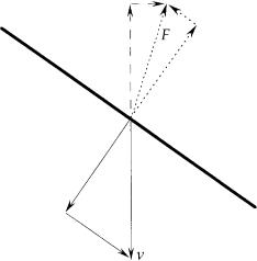
If you take a thin wire, hold it vertically, and drop it in a viscous medium, it falls straight down at some velocity, v. If, instead, you drop it horizontally, it falls straight down at about half that velocity, v/2. The viscous drag on the wire (the force per unit velocity that resists its motion) depends on the orientation: it is about twice as large when the wire moves sideways than when it moves lengthwise. As a consequence, if you drop the wire slantwise, say tilted downward to the right, it falls slantwise to the right. A formal analysis of a closely related problem, in which a wire is held slantwise and pulled straight downward, is shown in Fig. 6.1.
E. coli carries out this experiment by wrapping the wire into a helix and turning it about the helical axis, as shown, for example, in Figs. 5.4 and 5.5.The helix behaves like a series of wire segments pulled downward or upward, slantwise, in such a way that the forces generated by each segment in a direction parallel to the helical axis add up, providing the thrust that moves the cell body forward. If the cell (with its flagella) swims at a constant speed (does not accelerate or decelerate), it does not experience any net force; therefore, the thrust generated by the rotating helix must be balanced by the drag on the cell body. The same argument applies to rotation: the torque exerted by the flagellar motors on the filaments must be balanced by counterrotation of the cell body. However, since the body is relatively large, it turns relatively slowly. So when E. coli swims, the flagellar bundle spins one way on the order of 100Hz, while the cell body rolls the other way on the order of 10Hz; the cell with its flagella moves forward at speeds of order 10 body lengths per second. For a human being, 10 body lengths per second is about 40 miles per hour!
Reynolds Number |
51 |
FIGURE 6.1. A thin wire held slantwise and pulled downward through a viscous medium at velocity v. This velocity can be decomposed into components perpendicular to the wire and parallel to the wire, as shown below the wire. The drag due to the perpendicular component is twice as great per unit velocity as the drag due to the parallel component, as shown by the dotted lines above the wire. The net drag is F. It is not vertical but is tilted to the right, so it has a horizontal as well as a vertical component, as shown by the dashed lines. The horizontal component tends to move the wire to the right. If the wire were a segment of a rotating helix, this component would provide thrust. The vertical component opposes v, and thus determines the power required to move the filament. If the wire were a segment of a rotating helix, this component would contribute to the torque required to rotate the helix. For the orientation shown (55 degrees from vertical), the ratio of the horizontal to the vertical components (0.354) is maximum.
Reynolds Number
In a viscous medium, the ratio of the forces required to accelerate masses (inertial forces) to the forces required to generate shear (viscous forces) is called the Reynolds number, R. For a swimming creature, R = lvr/h, where l is the size of the creature, v is its velocity, r is the density of the medium, and h is the viscosity of the medium (a coefficient that characterizes its resistance to shear). For E. coli swimming full speed in water, R ª 10-5 (1/100,000). For a human paddling slowly in a swimming pool, R ª 105 (100,000). We are much bigger (l is much bigger) and we
52 6. Physical Constraints
move much more rapidly (v is much bigger). So, in a certain sense, our experience in water differs from that of E. coli by a factor of 1010. Our inertia is large, and it is easy for us to push off and coast from one side of the pool to the other. If you want to model what life is like for E. coli on a larger scale (by scaling up l and/or v), then you also must scale up h (work with a highly viscous medium). So use glycerol or corn syrup or a thick silicone oil, and don’t move things too rapidly. This restriction was not clearly understood until the work of Ludwig (1930), whose contribution was forgotten by the time the problem was taken up again by Taylor (1952).
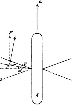
Ludwig noted a remarkable thing about motion at a low Reynolds number. If a pattern of displacements is reversed in time (neglecting diffusion), all elements of the system return to their initial positions, cell and fluid alike. The rate at which these displacements are carried out does not matter. Ludwig illustrated this point by imagining a creature with two rigid oars attached to the cell body by hinges, as shown in Fig. 6.2. The organism strokes its oars rapidly downward and returns them slowly upward. At a low Reynolds number, the cell body moves rapidly upward and then slowly downward, returning to its initial position. At a high Reynolds number, on the other hand, it moves farther during the power stroke than during the recovery stroke. There are microscopic unicellular algae that look somewhat like this cell (e.g., Chlamydomonas). However, they move their flagella in different ways during the power and recovery strokes: far from the cell body during the power stroke and close to the cell body during the recovery stroke (as in the human breast stroke). This motion is cyclic but not reciprocal; that is, the pattern is not reversed in time. Therefore (as Ludwig noted), it works at a low Reynolds number. The flagellar motion exhibited by E. coli also is cyclic: as long as the flagellar filaments turn steadily counterclockwise, the cell swims steadily forward.
Vivid images of this world were evoked by Purcell (1977) in an article titled, “Life at low Reynolds number.” Suppose, for example, that you are immersed in a swimming pool full of molasses and are allowed to move parts of your body no faster than the hands of a clock? According to Purcell, “If under those ground rules you are able to move a few meters in a couple of weeks, you may qualify as a low Reynolds number swimmer.” This world, while rather baffling to us, is one that E. coli knows intimately.
Diffusion 53
FIGURE 6.2. An organism propelled by two rigid oars, according to Ludwig (1930, Fig. 2). The oars move up and down between positions 1 and 2.A microscopic organism of this kind would just jiggle up and down. A macroscopic one, on the other hand, could swim by pulling the oars rapidly downward and returning them slowly upward. The arrows and
Greek symbols in the figure relate to Ludwig’s analysis of the problem, not examined here.
Diffusion
It is more difficult to model the utterly random motion due to thermal agitation. Whereas one can study the motion of macroscopic objects at low Reynolds numbers by working in highly viscous media, it is difficult to scale up a diffusion coefficient. There are no liquids with viscosities much lower than that of water, and work in gases is not practical because of perturbations due to gravity, notably, sedimentation and convection. It is easier to use a microscope and think small.The major take-home lesson is this: diffusive transport over small distances is very efficient, while diffusive
54 6. Physical Constraints
transport over large distances is very inefficient. Diffusion times increase as the square of the distance. Thus, a small molecule in water can diffuse the width of E. coli (1 mm) in a few milliseconds. To diffuse the width of your finger (1.5cm), it takes about a day.
To see how this comes about, consider a one-dimensional random walk. An ensemble of small creatures live on the x-axis and step with probability 1/2 to the right (+) or to the left (-) a distance d every t seconds. A record of the progress of six such creatures after 10 steps would look something like this:
Steps taken |
Distance moved |
Distance squared |
---+--+--- |
-6d |
36d 2 |
++-+++---- |
0 |
0 |
+++-++--+- |
+2d |
4d 2 |
-------+++ |
-4d |
16d 2 |
-+-+-++--+ |
0 |
0 |
++-+-+-+-+ |
+2d |
4d 2 |
This list was generated by flipping a coin. Some creatures drift to the right, some to the left, but on average—one needs a larger list to prove this—they go nowhere. The mean displacement for this list is x = -d, where the brackets denote an ensemble average. But the creatures have spread out, and one can get a measure of this by computing their mean-square displacement (the average of the square of the displacement), which for this list is x2 = 10d2. The mean-square displacement increases linearly with the number of steps (see Berg, 1993, Chapter 1). For example, if you break this list in half and treat it as 12 creatures each taking five steps, you will find a mean-square displacement 6.3d2, which is about half as large as before. Now, if t is the running time for the experiment, the number of steps is t/t, so x2 = (t/t)d2 = (d2/t)t. The coefficient that characterizes step distances and step times is commonly written D = d2/2t, which gives x2 = 2Dt. This is the mean-square displacement for one dimension. Similar equations can be written for motion along the y and z axes. If the motions along the x, y, and z axes are statistically independent (the usual case), then the mean-square displacement in two dimensions is x2 + y2 = 4Dt, and the mean-square displacement in three dimensions is x2 + y2
+ z2 = 6Dt.
D is called the diffusion coefficient. It depends on the size of the particle (and to a lesser extent, its shape), the viscosity of the medium in which the particle is immersed, and the temperature.
Diffusion 55
For a small molecule in water D ª 10-5 cm2/sec = 10-9 m2/sec. So when I said a small molecule can diffuse the width of E. coli in a few milliseconds, what I really meant was t = x2 /2D ª (10-6 m)2/(2 ¥ 10-9 m2/sec) = 5 ¥ 10-4 sec. That is, if a molecule starts out at one side of the cell at time 0, the chances are pretty good that it will reach the other side within a millisecond. But the chances are equally good that it will have gone a similar distance in the opposite direction (neglecting the impediment of the cell wall). The diffusion coefficient characterizes a spreading distance, not a velocity. Indeed, there is no such thing as a diffusion velocity: because of the square, it takes a set of diffusing particles four times as long to spread twice as far. To diffuse 1.5cm, t = (1.5 ¥ 10-2 m)2/(2 ¥ 10-9 m2/sec) = 1.1 ¥ 105 sec = 1.3 days. For globular-shaped particles in water, D is proportional to T/ah, where T is the absolute temperature, a is the radius of the particle, and h is the viscosity of water (which is smaller at higher temperatures).
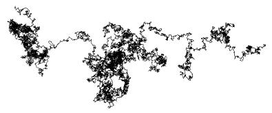
A simulation of a two-dimensional random walk is shown in Fig. 6.3. Diffusive transport over small distances is very efficient: the plotter pen tended to explore some regions of space rather thoroughly, returning to the same point many times before wandering away for good. Diffusive transport over large distances is very inefficient: when the plotter pen did wander away, it did so blindly, with no inkling of where it had been or where it might go. As a result, some parts of the plot are filled in, and others are quite empty.
FIGURE 6.3. An x,y plot of a two-dimensional random walk of 21,537 steps. At each step a computer flipped a coin twice and moved the plotting pen diagonally, to the right upward for +,+; to the right downward for +,-; to the left upward for -,+; and to the left downward for -,-. The first 18,050 steps of this walk are shown in Berg (1993, Fig. 1.4).
56 6. Physical Constraints
As we have seen,when E.coli swims,it picks directions at random. Therefore,it also diffuses.The step lengths for a motile cell are much longer than those due to thermal agitation, but they do not occur as often. The translational diffusion coefficient for a wild-type cell is much larger than that for a nonmotile cell, roughly D = 4 ¥ 10-10 m2/sec, as compared to 2 ¥ 10-13 m2/sec. But even a smoothswimming mutant executes a random walk, because rotational diffusion carries the cell off course. The same kind of coin-flipping experiment with increments in angle yields a mean-square angular displacement about one axis q2 = 2Drt, where Dr is a rotational diffusion coefficient. For globular-shaped particles in water, Dr is proportional to T/a3h. As noted earlier, this mechanism carries E. coli off course by about 90 degrees in 10 seconds. As a result, the translational diffusion coefficient for the smooth-swimming mutant works out to about D = 2 ¥ 10-9 m2/sec, roughly 5 times that of the wild-type cell.To learn more, see Berg (1993, Chapters 4, 6).
Diffusion of Attractants or Repellents
Diffusion of attractants or repellents sets a lower limit on the distance (and thus the time) that a cell must swim to outrun diffusion (to reach greener pastures), as well as on the precision with which the cell, in a given time, can determine concentrations. Diffusion of attractants or repellents also determines the number of receptors of a given kind that the cell needs to carry out these measurements. If a cell remains in one place for time t, it will sample molecules that come from a distance of order (Dt)1/2, where D is their diffusion coefficient. If the cell swims at velocity v during time t, it will be displaced a distance of order vt. If it is to go far enough to find out whether life is getting better or worse, it must outrun diffusion. This implies vt > (Dt)1/2, or t > D/v2. For E. coli swimming 30 mm/sec, t > (10-9 m2/sec)/(3 ¥ 10-5 m/sec)2 ª 1sec. This time is approximately equal to the mean run length. Recall that when a cell responds to gradients of attractants or repellents, it tends to extend runs rather than shorten them. Presumably, it does this because it can learn more by doing so. Short runs are not very informative.
If attractants or repellents are absorbed by a moving cell, there are fewer available at the back than at the front, but the difference proves to be small (Berg and Purcell, 1977). Nevertheless, this difference is large enough to rule out a mechanism in which
Diffusion of Attractants or Repellents |
57 |
a rapidly moving cell compares counts in the front with those in the back, that is, in which it makes spatial comparisons. The apparent gradient generated by the motion is several hundred times steeper than gradients encountered during chemotaxis. As a result, were the cell to choose a new direction at random, any direction would be deemed favorable. In other respects, however, the spatial mechanism is viable: a stationary cell could obtain the precision required to detect small differences in concentrations at its poles, simply by counting molecules for a relatively long time. The moving cell does so by comparing counts as a function of time, that is, by making temporal comparisons.
It is possible to estimate the time required for a cell to measure the concentraton of molecules with a given precision.Assume that the cell can count molecules in its own volume, a3, where a is its linear dimension (10-6 m). The result of one such count is a3C, where C is the mean concentration of molecules in its environment. Sampling of this kind is governed by the Poisson distribution, and the standard deviation is equal to the square-root of the mean (Berg, 1993, p. 90). Therefore, the uncertainty in the count is (a3C)1/2, yielding a precision (the standard deviation divided by the mean) of (a3C)-1/2. For E. coli in, say, 1 mM aspartate, (a3C)-1/2 ª [(10-6 m)3 (6 ¥ 1020 molecules/m3)]-1/2 = 0.04, or 4%. The cell can do better by waiting for the molecules that it has counted to diffuse away and for another set to diffuse in. If this happens, the two counts will be statistically independent. The required waiting time is of order a2/D, where D is the diffusion coefficient. If the cell continues this process for time t, the total count will increase by a factor t/(a2/D) = Dt/a2, yielding a final count DaCt, with precision (DaCt)-1/2. For t = 1sec, a = 10-6 m, and D = 10-9 m2/sec, Dt/a2 = 103, yielding a precision of about 0.1%.
To determine whether the concentration is going up or down, the cell has to make two such measurements and take the difference. It will not be able to make an informed decision unless this difference is larger than its standard deviation. Since things improve as t1/2, it would appear that the cell might work to arbitrarily high precision, simply by counting for very long times. But as we have seen, rotational brownian movement of the cell body sets an upper limit of order t = 10sec. To correct its course, the cell must deal with the recent past, not the distant past. So, for the counts to be large enough, C cannot be too small. For a cell swimming 30 mm/sec integrating counts over periods of 1sec, a precision of 0.1% (as estimated for 1 mM aspartate, above) is sufficient
58 6. Physical Constraints
for sensing a gradient with a decay length of about 2cm. For a more rigorous discussion of the counting problem, see Berg and Purcell (1977).
There is an additional wrinkle. The cell can only count molecules if they bind to a receptor. The chemotaxis machinery inside the cell monitors the occupancy of these receptors. A molecule of attractant diffuses around until it finds an empty binding site, sticks for a short time, and then diffuses away. The ratio of the offto the on-rates is known as the dissociation constant, Kd, which equals the concentration, in moles per liter, at which the receptor occupancy is one-half.This is the concentration at which the receptors are most sensitive to fractional changes in concentration. To work at concentrations large enough for adequate precision, the receptors for the best attractants (e.g., aspartate or serine) have dissociation constants in the micromolar range. If the on-rates are diffusion limited, the dwell times (inverse off-rates) turn out to be about 10-4 sec. Therefore, some device within the cell must compute the fraction of time that a receptor is occupied. Molecules continuously bind to the receptor and diffuse away, sticking for a time quite short compared to the time required for the cell to complete a single measurement.
How many receptors of a given kind must a cell have to count a substantial fraction of the molecules that impinge on its surface? As evident from the preceding discussion and Fig. 6.3, it takes a given molecule a relatively long time to reach a specific region of space. But once it is there, it explores that region rather thoroughly. Once a molecule encounters the cell surface, it tends to collide with that surface hundreds or thousands of times before it wanders away for good. As a result, it has an excellent chance of encountering a specific binding site. One can show that E. coli can do about half as well with a few thousand receptors of a given kind as it would do were its entire surface dedicated to that one specific task (see Berg, 1993, pp. 30–33). As a result, the cell has room for many different kinds of receptors (or transporters), each working at reasonable efficiency. This is a boon, not a constraint. Without benefits of this kind, microscopic life would not be possible.
Recapitulation
Since E. coli is more familiar with this world that we are, let me repeat. Flagellar filaments are long, thin, and helical, because
References 59
motion is dominated by viscous rather than inertial forces: thrust is generated by viscous drag. A cell is unable to swim in a straight line, because rotational perturbations due to brownian movement knock it off its path. Long runs are more effective for exploring the environment than short ones, because they allow the cell to outrun diffusion of the molecules that it needs to count. Rapidly moving cells must sense chemical gradients temporally rather than spatially, because comparisons between concentrations in front or behind are overwhelmed by diffusive currents due to their motion. Finally, the precision with which a cell can make temporal comparisons is limited by statistical fluctuations. The counting statistics improve with the square root of the product of the concentration and the integration time. A chemical cannot be sensed at an arbitraily low concentration because the integration time required would be prohibitively long.
References
Berg, H. C. 1993. Random Walks in Biology. Princeton University Press, Princeton.
Berg, H. C., and E. M. Purcell. 1977. Physics of chemoreception. Biophys. J. 20:193–219.
Brown, R. 1828. A Brief Account of Microscopical Observations on the Particles Contained in the Pollen of Plants; and on the General Existence of Active Molecules in Organic and Inorganic Bodies. Richard Taylor, London.
Ludwig, W. 1930. Zur Theorie der Flimmerbewegung (Dynamik, Nutzeffekt, Energiebalanz). Z. Vgl. Physiol. 13:397–504.
Purcell, E. M. 1977. Life at low Reynolds number. Am. J. Phys. 45:3–11. Taylor, G. I. 1952. The action of waving cylindrical tails in propelling
microscopic organisms. Proc. R. Soc. Lond. A 211:225–239.
This page intentionally left blank