

4
Individual Cells
Tracking Bacteria
If one looks through a microscope at a suspension of cells of motile E. coli, one is dazzled by the activity. Nearly every organism moves at speeds of order 10 body lengths per second. A cell swims steadily in one direction for a second or so (in a direction roughly parallel to its body axis), moves erratically for a small fraction of a second, and then swims steadily again in a different direction. Some cells wobble from side to side or tumble end over end. A few just seem to fidget. Given enough oxygen, the cells do this forever, even as they grow and divide. Near the middle of such a preparation, cells rapidly appear and disappear as they move in and out of focus, while at the bottom or the top they tend to spiral along the glass surface, clockwise (CW) at the bottom, counterclockwise (CCW) at the top. The speed at which the cells swim depends on how they have been grown (two to three times faster when grown on a rich medium than on a simple one), on the ambient temperature (twice as fast at body temperature than at room temperature), and on how they have been handled. Flagella are fragile and break if suspensions are subjected to viscous shear, particularly when cell densities are high (as in a centrifuge pellet). If one tries to resuspend such a pellet by flicking the centrifuge tube with one’s finger, cell motility is noticeably degraded.
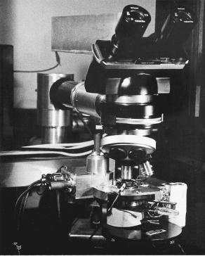
My interest in quantifying this motion was sparked in 1968 by a conversation with Max Delbrück, who bemoaned the fact that he did not know how to “tame” bacteria. By “tame,” I finally realized, he meant monitoring the behavior of individual cells. This was what he was doing in his work on growth of the spore-bearing stalk of the fungus Phycomyces, simply by using a telescope. So I built a microscope that could follow the motion of individual cells of E. coli in three dimensions (Fig. 4.1). In essence, this is a
31
32 4. Individual Cells
FIGURE 4.1. The tracking microscope, circa 1974. The lenses, mirrors, and fiber-optic assembly used to dissect the image of a cell was built into the rectangular box extending back from the top of the binocular. Just below the objective is a thermostatted enclosure containing a small chamber in which the bacteria were suspended, mounted on a platform driven by three sets of electromagnetic coils (similar to loudspeaker coils) built into the assembly at the left. (From Berg, 1978, Fig. 2).
three-dimensional direct current (DC) servo system in which errors in the position of the image of a bacterium sensed at the top of the microscope (where one normally places a camera) are used to control the position of a small chamber holding a cell suspension, so that the image (and hence the bacterium) remains fixed in the laboratory reference frame. To follow the movement of the bacterium, all one has to do is write down the position (the x, y, and z coordinates) of the chamber. It’s rather like following the progress of a worm in a bucket of soil by moving the bucket
Tracking Bacteria |
33 |
so that the worm remains fixed in the reference frame of one’s garden. The accelerations are so slight that neither the bacterium nor the worm knows that it is being manipulated. This is a nonperturbative measurement.
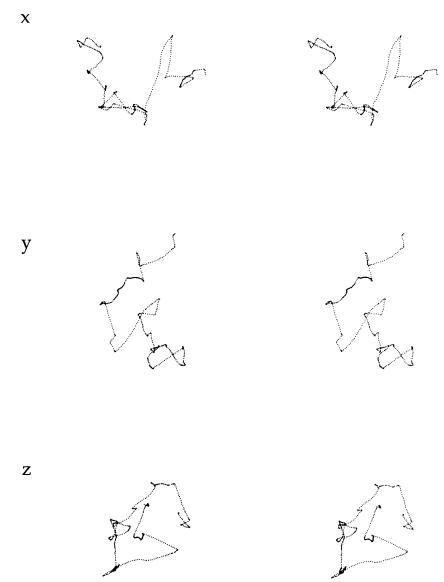
Tracking is fun. When viewed through the microscope, the cell being followed changes its orientation or its mode of vibration but remains in focus at a fixed point. The other cells drift this way and that, in apparent synchrony. One of my favorite tracks is shown in Fig. 4.2: three stereo views of the same data set, representing about 30 seconds in the life of a wild-type (behaviorally competent) cell, swimming in the absence of any chemical gradients. E. coli just wanders around, trying new directions at random. The smooth segments of this random walk are called “runs,” and the erratic intervals are called “tumbles.” During runs, the cell moves along a reasonably smooth track. During tumbles, it moves erratically in place. After a tumble, it sets off again along another smooth track, but in a new direction chosen nearly at random. Computer analysis of such data showed that run intervals are distributed exponentially, with short intervals the more probable. The lengths of successive intervals are not correlated. This is just what one finds for intervals between clicks of a Geiger counter, where emissions from a radioisotope occur with a constant probability per unit time. Not only are short intervals the more probable, they appear to be bunched. What one often calls a tumble when viewing cells by eye actually is a sequence of short runs and tumbles (which is why, in the original work, I used the word “twiddle” rather than “tumble”).The mean run interval is about 1 second, varying somewhat from cell to cell. Tumble intervals also are distributed exponentially, with a mean of about 0.1 second, but this value is the same from cell to cell.
Figure 4.3 shows the swimming speed of the cell of Fig. 4.2. The bars indicate tumbles logged by the computer. It takes the cell a while to get up to speed following a tumble, but the terminal speeds are nearly identical. The reasons for this are discussed in the next chapter.
If cells were to choose new directions at random, the distribution of turn angles would follow a sine curve, with a mean of 90 degrees. In dilute aqueous media, there is a slight preference for the forward direction, and the mean is 68 degrees. But it only takes a cell a few tumbles to forget where it has been. It does not know where it is going.
34 4. Individual Cells
FIGURE 4.2. Three stereo plots of a track of one cell of E. coli strain AW405 (wild type for chemotaxis) viewed along the x, y, and z axes (top, middle, and bottom, respectively). To see a given plot in three dimensions, look at the left image with your left eye and the right image with your right eye, and relax your eye muscles so that the two images overlap. A stereoscope (a pair of lenses) helps. The cell was tracked in Adler’s motility medium at 32°C for 29.5 seconds, and the x, y, and z outputs were digitized 12.6 times per second. The largest span across the track (e.g., from top to bottom in the middle plot) is 106 mm. There were 26 runs and tumbles; the longest run was 3.6 seconds. The mean speed was 21.2 mm/sec. (Data from Berg and Brown, 1972, Fig. 1.)

Response to Spatial Gradients |
35 |
FIGURE 4.3. The speed of the cell whose track is shown in the previous figure. Tumbles occurred during the intervals shown by the bars. A stripchart record of the output of an electronic speedometer was divided into three parts, which were stacked on top of one another. (From Berg and Brown, 1972, Fig. 2.)
Response to Spatial Gradients
How, then, do cells respond to gradients? To answer this question, we inserted one of Adler’s capillary tubes (Fig. 3.5) through the side wall of a tracking chamber and followed cells in gradients of serine and aspartate. Given Engelmann’s demonstration of the shock reaction, we had expected that E. coli would shorten runs that are unfavorable. The result proved to be exactly the opposite. E. coli extends runs that are favorable (that carry cells up the gradient of an attractant) but fails to shorten runs that are not (that carry cells down such a gradient). The random walk of Fig. 4.2 becomes biased, and the bias is positive. The bias is large enough to enable a cell to move up a gradient at about 10% of its run speed. There is no correlation between the change in direction generated by a tumble and the cell’s prior course; tumbles have precisely the same effect whether a cell swims in a gradient or not, they just occur with different frequencies. Thus, if life gets better, E. coli swims farther on the current leg of its track and enjoys it more. If life gets worse, it just relaxes back to its normal mode of behavior. E. coli is an optimist.
36 4. Individual Cells
Response to Temporal Gradients
The next question was whether cells respond to spatial or temporal stimuli. That is, is a favorable run extended because the cell finds more attractant near its nose than near its tail, or because the concentration goes up as it moves along? Recall that the answer for Chromatium was temporal. When Engelmann passed his hand between the light source and the microscope stage, all the cells in the field of view backed up; when he exposed cells in a hanging drop to carbon dioxide, they backed up regardless of their orientation relative to the surface of the drop. We decided to answer this question for E. coli by a method that did not expose cells to spatial inhomogeneities, such as those encountered during mixing of chemicals or diffusion into the surface of a drop. We found an enzyme, available commercially, that would convert an innocuous substance into a chemical attractant. The reaction was reversible, so alternatively the attractant could be destroyed. Thus, no matter where a cell might be or where it might be headed, it would always find the concentration of the attractant rising or falling. When the attractant was generated, all the runs got longer. When it was destroyed, the cells failed to respond. The response to the positive temporal gradient was large enough to account for the results obtained in spatial gradients (Brown and Berg, 1974).
The question of whether cells respond to spatial or temporal stimuli had been considered earlier in a simpler way by Macnab and Koshland (1972), who rapidly mixed suspensions of cells and attractants and recorded the response under a microscope using stroboscopic illumination. Cells suddenly exposed to a positive step of serine (0 to 0.8 mM) swam smoothly (without tumbling) for up to 5 minutes. Cells exposed to a negative step (1 to 0.24 mM) tumbled incessantly for about 12 seconds. These experiments showed that E. coli (actually Salmonella) senses temporal stimuli. Technically, this was true not because the cells responded, but because the responses to positive and negative steps were different (of opposite sign), even though the spatial homogeneities to which the cells were exposed during mixing were roughly the same. E. coli does not encounter temporal stimuli of this magnitude when swimming in spatial gradients in nature. Unless there is a strong source (e.g., a fine capillary tube) and a strong sink (e.g., a large surrounding pond), spatial gradients are rapidly smoothed out by diffusion. In any event, cells do not swim fast enough to
References 37
generate large temporal stimuli. Such stimuli saturate the response: in the mixing experiments, cells either swam without tumbling or tumbled incessantly, although much longer in the former than in the latter case. What one measures is the time required for the cells to recover (i.e., to return to a mode in which they run and tumble). However, such stimuli have proved quite useful for probing the chemotaxis machinery.
References
Berg, H. C. 1978. The tracking microscope. Adv. Opt. Elect. Microsc. 7:1–15.
Berg, H. C., and D. A. Brown. 1972. Chemotaxis in Escherichia coli analysed by three-dimensional tracking. Nature 239:500–504.
Brown, D. A., and H. C. Berg. 1974. Temporal stimulation of chemotaxis in Escherichia coli. Proc. Natl. Acad. Sci. USA 71:1388–1392.
Macnab, R. M., and D. E. Koshland, Jr. 1972. The gradient-sensing mechanism in bacterial chemotaxis. Proc. Natl. Acad. Sci. USA 69: 2509–2512.
This page intentionally left blank