the variables) then the dual model would also be in standard form as a minimisation subject to all ‘ ’ constraints.

The decision procedure, which we illustrated in Example 2.3, shows that the optimal solution to the dual model gives an attainable upper bound on the optimal objective value of the primal model. Hence, if both the primal and dual models have finite optimal solutions, their optimal objective values are the same (there is no ‘duality gap’). The optimal values of the dual variables are known as the dual values of the corresponding constraints in the primal model. It might be the case that the dual model is infeasible in which case the primal model may have no bound on its optimal objective value (it is said to be unbounded) or it might itself be infeasible. If the primal model is unbounded then we can produce no upper bound on the primal objective value and therefore the dual model can have no solution and must be infeasible. All these results are part of the duality theorem of LP. The variables in the dual model have important economic interpretations in many applications as well as having computational applications. Of course duality is also of mathematical interest since there is a symmetry between the primal and dual models. The dual of the dual model is the primal model (Exercise 2.6.3).

We should point out that the duality between LP models, which we have exhibited here, is different from the logical duality which we discussed in Chapter 1.

2.1.2 A Geometrical Representation of a Linear Programme

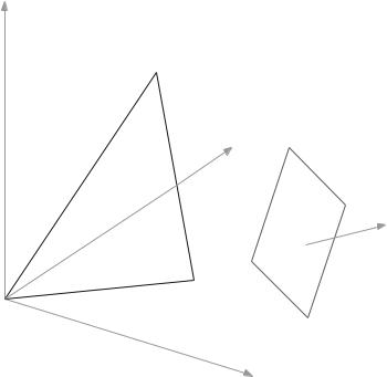
The variables in an LP model can be interpreted as the coordinates of points in space. The dimension of the space is equal to the number of variables in the model. We illustrate this by giving a geometrical representation of the model in Example 2.1.

As all the variables are non-negative we restrict ourselves to the non-negative orthant. The constraints, in this example, restrict us to the triangular region A, B, C. This is known as the feasible region. Particular values for the objective function lie on planes with the orientation of that shown. Increasing values of the objective function arise as the planes are moved in the direction shown. However, we need a plane that intersects the feasible region. This happens, for this example, when an objective plane intersects the vertex B of the feasible region, whose coordinates x1 = 1, x2 = 2, x3 = 0 therefore give the optimal solution (Fig. 2.1).

In this particular example the feasible region is non-full dimensional, i.e. not of a dimension equal to the number of variables. It illustrates a number of features of the geometrical representation of LPs which generalise.

The feasible region is a polytope. These are regions of space, in any number of dimensions, whose boundaries are hyperplanes, i.e. lines, planes or higher dimensional generalisations. They are of dimension one less than the dimension of the polytope. In this example the polytope of the feasible region is closed. In general, however, LP polytopes can be open, as illustrated by Example 2.5. Such polytopes are sometimes referred to as polyhedra. For an LP polytope the feasible region can be characterised by its boundaries, known as its facets or, alternatively by its vertices.

C (0,3,3)

x3

x2

objective plane

x1

Fig. 2.1 A non-full dimensional LP model

Different values of the objective function will be represented by hyperplanes in the space. Moving to parallel hyperplanes in a direction orthogonal to the hyperplanes will increase the objective value and in the other direction decrease the objective value. As in the example the optimal solution will normally correspond to where an objective hyperplane intersects a vertex of the feasible region. However, it may be the case that the orientation of the objective hyperplane is such that there are alternative optimal solutions not at vertices. But among the alternative optimal solutions there will still be vertex solutions (so long as the model is not infeasible or unbounded).

Some of these different features of LP models are illustrated in examples below and in exercises in Sect. 2.6. We emphasise again that our purpose is to explain the nature of LP in so much as is necessary for the understanding of IP. There are many other texts that give a rigorous mathematical derivation of these properties, some of which are referenced in Sect. 2.5.

We give some other examples of LP models

Example 2.4 A full-dimensional LP model

Maximise

This is illustrated in Fig. 2.2. Note that this model is in standard form.

x3

C(0,7/3,1/3)

A(0,0,3/2)

x2

D(1/2,5/2,0)

E(0,2,0)

O(0,0,0)

B(3,0,0) x1

Fig. 2.2 A full-dimensional LP model

It can be seen that the feasible region has six vertices O, A, B, C, D and E with their coordinates marked. The orientation of the objective plane shows that

the (unique) optimal solution arises from vertex C giving the solution x1 = 0, x2 = 73 , x3 = 13 , objective = 383 .

Example 2.5 An LP with an open feasible region

Minimise

x1, x2 R

Note that this model is also in standard form. It is illustrated in Fig. 2.3. (When we have a minimisation model we adopt the convention that dual values on ‘ ’ constraints are non-negative, whereas dual values on ‘ ’ constraints are non-positive, in contrast to these conventions being reversed for maximisation models.)

x2

D

C

A(0,5/2)

B(9/5,8/5)

x1

Fig. 2.3 An LP model with an open feasible region

The optimal solution occurs at vertex B giving x1 = 95 , x2 = 85 , objective = − 15 . If, however, the objective had been (say)

Minimise

− 3x1 + x2 (2.36)

then the model would have been unbounded since feasible solutions of everdecreasing objective value could be found.

A polyhedron with an open feasible region (in any number of dimensions) is characterised by its vertices and its extreme rays. In the example AD and BC are extreme rays. If an LP is unbounded then the unboundedness is represented by an extreme ray such as BC, for this example, with objective (2.36). Note that points on this extreme ray give ever-decreasing values for objective (2.36).

It has already been remarked that if an LP is unbounded the corresponding dual model is infeasible, i.e. the decision procedure illustrated in Example 2.3 will produce no lower bound (in the case of a minimisation) on the objective (see Exercise 2.6.5). We give the dual model to Example 2.3 (with objective (2.36)).

Example 2.6 An infeasible LP model

Maximise

In Fig. 2.4 it is shown that the constraints above are self-contradictory.

In order to satisfy constraint (2.38) (and the non-negativity constraints) we have to lie in the upper open region, but in order to satisfy constraint (2.39) we have to lie in the lower triangular region. These regions have no points in common.

Note that the property of infeasibility is independent of the objective function. If a model is infeasible it has no solutions irrespective of the objective.

It has already been remarked that if a model is unbounded its dual must be infeasible. Exercise 2.6.6 is to show that the dual of Example 2.6 (which is infeasible) is Example 2.5 with objective (2.36) (which is unbounded). It was also, however, remarked that if a model is infeasible there is another possibility: its dual may also be infeasible. Exercise 2.6.7 demonstrates this.

The method of solving LP models by the elimination of existential quantifiers, illustrated in Example 2.3, can be regarded in a geometrical context as a method of projection. Each time a variable is eliminated the model is projected down to an equivalent model in a space of one less dimension. The method can be valuable in reformulating both LP and IP models.

LP models arise in many contexts such as production, distribution, blending, oil refinery scheduling and chemical processing to name only a few. Models can involve millions of constraints and variables. In Sect. 2.5 references are given to comprehensive sources which discuss practical applications.

Before discussing IP we should point out that there are important classes of apparent IP models which can be solved as LPs as this leads to integer values for the