14 1 An Introduction to Logic

Using Fig. 1.1 it is easy to verify, for example, De Morgan’s laws. The region outside the two circles is modelled by A B. It is easy to see that this is also the intersection of the complement of A with the complement of B which is modelled

by A · B.

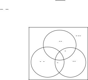
Figure 1.2 demonstrates how extended disjunctive normal form can model a statement.

Fig. 1.2 A second Venn diagram

All eight disjoint regions are modelled by the eight conjunctive clauses made up from A, B, C and their negations. A is represented by the top circle, B by the left circle and C by the right circle. We have used the symbols A, B, C in two senses. On the figure they represent regions with the set operations ‘ ’, ‘∩’ and ‘−’ (complement) applied. In the propositional calculus statements they represent atomic statements (indicating membership of the corresponding region) with the corresponding connectives ‘ ’, ‘·’ and ‘−’ (‘not’) (using the same symbol as for the set complement).

1.4 The Predicate Calculus

While the propositional calculus is sufficient for many purposes it is not sufficient to formalise all mathematics. The predicate calculus was created for this purpose. In this system statements can be made about objects by means of predicates, e.g. P(x, y). P(x, y) could stand for a statement such as

If the variables x and y are set to constants such as ‘James’ and ‘Mary’ we have the statement P(J ames, Mar y) , which will be true or false meaning

Predicates can be of one, two, three or any number of variables. The process of setting variables to constants is known as instantiation. Each variable in a predicate has a domain of possible values. In addition to the predicates we have the connectives of the propositional calculus for combining them into compound predicates. Instantiation of all the variables in the predicates of an expression converts it to a statement in the propositional calculus.

For example if we have the statement

we might instantiate it to

so long as a, b and c were in the appropriate domains. Its truth, or otherwise, will depend on the truth values of the atomic statements in the standard way.

1.4.1 The Use of Quantifiers

A major strength of the enhanced expressive power of the predicate calculus is the use of quantifiers. These are written as ‘ ’ and ‘ ’. ‘ ’ means ‘for all’ and ‘ ’ means ‘there exists’. If, for example, we have x Q(x) this means ‘for all objects in the domain of x, Q(x) is true’. This can then be regarded as an atomic proposition of the propositional calculus. Likewise the statement x Q(x) means ‘there exists an object in the domain of x for which Q(x) is true’.

The following statements are usually stipulated in the form of axioms of the predicate calculus but we simply state them as valid deductions and equivalences in our informal treatment. They obviously accord with the meanings we have given to the quantifiers. They enable us to manipulate and translate statements in the calculus (into, for example, normal forms). As before we assume that the objects (constants) a, b, c, . . . fall within the permitted domains of the variables x, y, z, . . . where they are substituted

Note that we are using the symbol ‘˜’ as an alternative to ‘−’ solely for notational convenience. Equations (1.56) and (1.57) are obviously generalisations of De Morgan’s laws.

If the domain of a predicate is finite (e.g. a, b, . . . , n) then we can use the connectives ‘·’ and ‘ ’ in place of ‘ ’ and ‘ ’, e.g.

Besides the ability to quantify over infinite domains (e.g. the natural, real or rational numbers) the new notation also has great advantages in helping us to create clear and succinct expressions even if the domains are finite. It can be very useful in modelling as is illustrated in Chapter 3.

The predicate calculus is sometimes referred to as ‘first-order theory’ since it allows us to quantify the objects within predicates but not ‘higher order’ objects such as the predicates themselves.

Each quantifier has a scope over which it applies, e.g.

is itself a predicate of the variables y, z, s. The scope of x is the first disjunction of T and U and is indicated by bracketing them. It does not extend to W . The variable x is said to be bound by the quantifier. It is a dummy variable which could equally well be replaced by another variable and the meaning be unchanged. To save confusion it is clearer not to use such a variable elsewhere, beyond the scope of the quantifier. Variables that are not bound are said to be free. y, z, s are free in the above expression. Since W does not involve x there would be no ambiguity in extending the scope of x to the whole expression by moving the last bracket after

Uto the end of the expression.

1.4.2Prenex Normal Form

Using (1.56) and (1.57) we can move all the quantifiers to the beginning of an expression creating what is known as prenex normal form. We illustrate this by an example. The expression which is quantified will be known as the core.

Example 1.5 Transform the following expression into prenex normal form and the core into DNF:

Note that only variables x1,x2,x3 and x6 are bound. Therefore the expression is itself a predicate of the free variables x4 and x5. We can successively transform (1.61) into

It is sometimes convenient to allow one quantifier to apply to a group of variables, e.g. x1 x2 can be written as x1 x2. Similarly for . Also it can easily be verified that x1 x2 means the same as x2 x1. Similarly for .

When reading a statement such as (1.65) it must be remembered that the quantifiers should be read from left to right. The left most quantifier applies to the statement (including quantifiers) to its right and so on. However, the order of andcannot be reversed. x y P(x, y) does not mean the same as y x P(x, y). To illustrate this let us take the domain of x and y as the integers and P(x, y) as the relation x y. The first statement is clearly not true in this interpretation since there is no integer which is smaller or equal to all the rest. However, the second statement is true in this interpretation since for any integer there is always an integer which is smaller or equal to it (e.g. itself). One might conveniently represent such an integer as xy indicating that it depends on the value of y, whereas for the first statement we

If the premise holds then for all y there is an x such that P(x, y), i.e. a particular, single, x serves the purpose for all the y. (For the positive integers, with the predicate ‘x y’ for example, 1 serves the purpose.) Hence for a particular y the conclusion will also be true since the specific x chosen for the premise will also serve the purpose.

In order to demonstrate the expressive power of the predicate calculus in a nonmathematical setting we consider the following example.

Example 1.7 Express the following statement using the predicate calculus:

and some o f the people all o f the time, but

you cannot f ool all o f the people all o f the time

Let the predicate P(x, y) be given the interpretation ‘x can be fooled at time y’. The statement can then be written as