If we have an objective then we have a MIP model. We solve this below. Alternative and better ways of formulating such logical problems (including this

example) are described in Sect. 3.3.

3.2 Disjunctive Programming

The logical connective that distinguishes IP from LP is ‘ ’. It has been seen that ‘˜’ simply transforms inequalities to other (strict) inequalities that are usually modelled by approximating a non-strict inequality. The ‘·’ connective is implicitly present in all LP models. If one negates an ‘=’ constraint (possibly first writing it as a conjunction of a ‘ ’ and a ‘ ’ constraint) one also obtains a disjunction. A disjunction is what requires the use of IP rather than LP. Hence the phrase ‘disjunctive programming’ is sometimes used to characterise this type of modelling.

Although we will be showing, in this chapter, how to model disjunctive programmes as IPs it would be possible to solve them (inefficiently) using the method described (for the theory of dense linear order) in Example 2.3. This is the subject of Exercises 3.7.9 and 3.7.10.

3.2.1 A Geometrical Representation

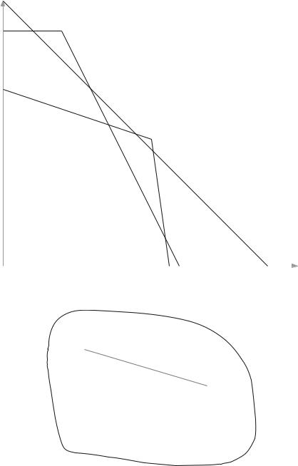
It is helpful to illustrate such models geometrically. We do this by representing Example 3.2 geometrically, in Fig. 3.1.

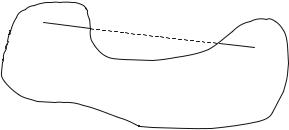
The boundaries of all the inequalities in (3.11) are marked and the feasible region, defined by the logical statement of inequalities, is OABCDEFGH. Note that this is really a Venn diagram (discussed in Sect. 1.3) as a result of the conjunctions and disjunctions. It is non-convex, unlike LP feasible regions that are always convex. A convex region is one in which any line between two points in the region always, itself, lies in the region. In Figs. 3.2 and 3.3 we illustrate the distinction.

Non-convex regions arise in a number of contexts. In non-linear programming the feasible regions may be non-convex and IP used, possibly approximating the feasible region by piecewise linear segments. IP has the advantage that it finds global, as opposed to local, optima as discussed in Sect. 2.3. If a region is non-convex, and approximated to in this way, then the convex region can be partitioned into the union of convex sets. Each convex set can be represented as the conjunction of LP constraints. Hence the overall region is a disjunction of these conjunctions giving us the constraints of a disjunctive programme. Therefore there is a close connection between IP and (non-convex) non-linear programming.

There is also a distinction to be made between convex and non-convex objectives. If the region above each contour, representing equal values of the objective function, is a convex set then the objective function is said to be convex. Minimising a convex function over a convex region (or equivalently maximising a concave function over a convex region) guarantees a global optimum from the LP relaxation. We therefore

It is instructive to view these solutions geometrically (in the space of x1 and x2) as is done in Fig. 3.4.

x2

4 A B

Fig. 3.4 A disjunctive programme

The optimal integer solution corresponds to vertex F in Fig. 3.4. Note that if this had represented a non-linear problem vertex H would have represented a local optimum (with a lower objective value). Traditional non-linear programming algorithms could well produce this solution. If we use branch-and-bound on the IP formulation then vertex H will correspond to another integer solution which might well be produced in the tree search before that at vertex F is found.

3.2.2 Mixed IP Representability

When is a problem representable as a MIP? We are going to restrict our attention to the possibility of modelling using bounded integer variables. In Chapter 2 it was shown that bounded integer variables can be expressed using only 0–1 integer variables. Hence we consider when it is possible to model, using continuous and 0–1 integer variables only. Such problems are sometimes referred to as bounded MIP representable but we will simply refer to these problems as MIP representable. We have seen that, in some circumstances, e.g. Example 3.2, it is possible to model a logical statement involving LP constraints as a conjunction of MIP constraints. But

we relied on some of the numerical bounds given in (3.1) in order to do this. If we know such bounds then it is possible to model the conditions in this way (possibly approximating strict inequalities if necessary). In some circumstances we do not know such bounds. Also the objective function may make the problem non-MIP representable. It may still be possible to model as a MIP but only if certain conditions apply, which we discuss here. Before doing this we give a simple logical condition which is not MIP representable.

Example 3.4 A non-MIP-representable condition

x, y R

Since we do not have bounds on the values of x and y we cannot, obviously, model this disjunction by introducing 0–1 variables. Even if we place single bounds on each variable (e.g. lower bounds of 0) the condition is still not representable.

Example 3.5 A MIP-representable disjunctive programme with an open feasible region

Minimise

x, y R

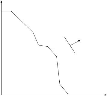
The feasible region is illustrated in Fig. 3.5. It can be seen that each clause in (3.32) gives rise to an open feasible region, as therefore does their union. However, Example 3.5 is MIP representable, unlike Example 3.4.

A MIP model representing Example 3.5 is Minimise

A

D

B

J

G

C

E

F H

I

Fig. 3.5 Disjunctive constraints with an open feasible region

subject to

δ1, δ2, δ3 {0, 1}

Constraint (3.41) forces at least one of δ1, δ2, δ3 to take the value 1. It can be verified that δ1 = 1 forces the constraints in the first clause of (3.32) to hold (but does not exclude the corresponding constraints holding in the other clauses). Similarly δ2 = 1 and δ3 = 1, respectively, force the second and third clauses to hold.

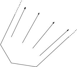
Why is Example 3.5 MIP representable while Example 3.4 is not? The reason is that the feasible region of Example 3.5 is the union of polyhedra with the same recession directions. A recession direction of a polyhedron (in this two-dimensional example) is a direction ( p, q) such that for any point (a, b) in the polyhedron all points (a +λp, b+λq) for all λ 0 are also in the polyhedron. Recession directions are drawn for a polyhedron in Fig. 3.6.

B

D

A

C

Fig. 3.6 Recession directions of an open polyhedron

Possible recession directions are those between the extreme rays AB and CD. In Fig. 3.5 it can be seen that the three polyhedra, whose union makes up the feasible region, have exactly the same recession directions since they all have extreme rays pointing in the same directions. We show below why this property makes the corresponding optimisation problems MIP representable. Before doing this, however, observe that Example 3.4 can be regarded as the union of two polyhedra x = 0 and y = 0 each of which have two, different, recession directions. Hence this example is not MIP representable.

If all the polyhedra, whose union makes up the feasible region of a problem, are closed then each of the polyhedra has no recession directions and the conditions are satisfied vacuously making the problem MIP representable. This is the case with Example 3.3.

Although all the above discussion has been illustrated by two-dimensional examples the concepts and results extend to any number of dimensions.

For completeness we solve the model resulting from Example 3.5.

The LP relaxation solution is

i.e. the same 0–1 variable is used for each constraint (open and closed) in a conjunctive clause.

Note that we can, in effect, confine ourselves to the same mi (or Mi for ‘ ’ constraints) which we would have used in the ‘closed parts’ of the corresponding polytopes.

For constraints that do not contain extreme rays of the polyhedra we can obtain bounds on the values of the variables in them and formulate the corresponding MIP constraints as described in Sect. 3.1.

Conversely, if we have a MIP representation of a model, then a typical constraint will be

x j R, δi {0, 1} j J, i I

Setting the δi to different values gives a series of parallel constraints.

Some, or all, of these constraints may represent closed hyperplanes. Some may be redundant in the presence of other constraints. However, if any represent open facets, of some of the component polyhedra in the implied disjunction, they must all represent open facets. What’s more they will be bounded by some extreme rays which must be parallel to the corresponding extreme rays in the other polyhedra in the implied disjunctions. This argument applies to all the constraints in (3.48). Hence the constraints in (3.48) represent a disjunction of polyhedra that are either all closed or, if not, have the same recession directions.

It remains to consider when the objective function, taken in conjunction with the constraints, still makes a problem MIP representable. If the objective is linear and expressed in the original variables (not involving the appended 0–1 variables) then there is no problem. This is the case with Examples 3.3 and 3.5. However, it may be the case that we wish to model a piecewise linear or a discontinuous objective. For example the non-linear expression given in Example 2.17 might have occurred in the objective function. It would then be replaced by a variable, with the necessary extra variables and constraints added to the model. The representability problem would then be the same as that for a logical system of constraints. If the objective is discontinuous then the situation may be more complex. This happens, for example, in the facility location problem discussed in Example 2.12. This problem is a special case of the fixed charge problem. We consider this problem in its simplest form in Example 3.6.