


4.3 Representation as an Integer Programme |
109 |
4.2 The Davis–Putnam–Loveland (DPL) Procedure
If a statement is not satisfiable then the empty clause is a prime implication (which absorbs all other implications rendering it the only one) and this will be obtained by successively applying resolution and absorption. Otherwise, if the empty clause is not obtained, then the statement is satisfiable. A satisfiable set of truth values can be obtained as follows:
1.(a) If a clause consists of a single literal X then set X = T. Similarly if a clause consists of a single literal X set X = F. Note: There will be no other clauses containing X or X by the application of absorption.
(b)If a literal is unnegated in all clauses within which it occurs set X = T and delete the clauses within which it occurs. (There may be alternative satisfying settings but this is sufficient if we are content only to find a satisfiable setting.) Similarly if a literal is negated in all clauses within which it occurs set X = F and delete all clauses within which it occurs. (Again there may be alternatives.)
(c)If a literal X is unnegated in some clauses and negated in others partition the clauses into two sets (i) and (ii).
(i)Set X = T and delete the clauses in which it is unnegated.
(ii)Set X = F and delete the clauses in which it is negated.
Each of the sets (i) and (ii) after this ‘branching’ is then treated as before by procedures (a), (b) and (c). It can be shown (Exercise 4.12.3) that at least one of the branches will result in a satisfiable set of truth values.
For, comparatively simple, Example 4.2 resolution and absorption resulted in (4.19): (a) sets X2 = F, X4 = T; (b) does not apply and (c) creates the settings (branching on, say, X1): (i) X1 = T, X3 = T and (ii) X1 = F, X3 = F.
After applying (b) we obtain the alternative sets of satisfying truth values
X1 = T, |
X2 |
= F, |
X3 |
= T, |
X4 = T |
(4.21) |
X1 = F, |
X2 |
= F, |
X3 |
= F, |
X4 = T |
(4.22) |
4.3 Representation as an Integer Programme
The satisfiability problem can be represented as the problem of deciding if an integer programme (IP) is feasible using the modelling methods described in Chapter 3. However, the satisfiability problem has a special structure as an IP which should be explained.
If the satisfiability problem is expressed in CNF then each (disjunctive) clause gives rise to a constraint. As in Chapter 2 we represent the truth or falsity of a literal
110 |
4 The Satisfiability Problem and Its Extensions |
X by a 0–1 variable x taking the value 1 or 0, respectively. If X occurs unnegated in a clause then x appears in the constraint. If it occurs negated then (1 − x) appears. The sum of these terms in the constraint must be 1.
For example the clause
|
|
|
|
(4.23) |
|
X1 X3 X4 |
|||
gives rise to the constraint |
|
|
||
(1 − x1) + x3 + x4 1 |
(4.24) |
|||
In more usual form this is written as |
|
|||
− x1 + x3 + x4 0 |
(4.25) |
|||
For Example 4.2 the full set of constraints is therefore |
|
|||
−x1 + x3 + x4 0 |
(4.26) |
|||
−x2 + x3 + x4 0 |
(4.27) |
|||
|
x1 |
− x3 0 |
(4.28) |
|
|
−x3 + x4 0 |
(4.29) |
||
−x1 + x3 − x4 −1 |
(4.30) |
|||
−x1 |
− x2 −1 |
(4.31) |
||
|
−x2 + x3 0 |
(4.32) |
||
|
x2 |
+ x4 1 |
(4.33) |
|
|
x3 |
+ x4 1 |
(4.34) |
|
The general form of such constraints is |
|
|||
r |
r+s |
|
||
− xi + |
xi (1 − r) |
(4.35) |
||
i=1 |
i=r+1 |
|
||
Models with such constraints are a special case of generalised set-covering problems (GSCPs). (GSCPs, in contrast to the set-covering problem mentioned in Chapter 2, have all coefficients 0, ±1 and general integer right-hand sides, with all constraints ‘ ’.) This special sort of GSCP can easily be converted to a set-covering problem (SCP) where all the coefficients and right-hand sides are 0–1 by substituting (1 − yi ) for xi in the first summation in (4.35). This then gives the constraints
r |
r+s |
|
yi + |
xi 1 |
(4.36) |
i=1 |
i=r+1 |
|
4.4 The Relationship Between Resolution and Cutting Planes |
111 |
Together with the extra constraints |
|
xi + yi = 1, i = 1, . . . , r |
(4.37) |
If (4.37) were converted to the ‘ ’ form then solutions satisfying the ‘=’ form could be sought by the choice of suitable objective function such as
|
r |
|
Minimise |
(xi + yi ) |
(4.38) |
|
i=1 |
|
If this objective can be minimised to r then (4.37) must be satisfied and the original problem is satisfiable.
However, for our purposes it suffices to consider satisfiability problems in the form of GSCPs.
4.4 The Relationship Between Resolution and Cutting Planes
We could solve the problems described above as IPs using the branch-and-bound method described in Chapter 2. However, it is worth pointing out that we can often, with benefit, reduce the size of such models first. The methods of reduction we use mirror resolution and absorption as described in Sect. 4.1. We illustrate this by reference to constraints (4.8) and (4.16).
If one constraint is implied by another it can be removed. This happens when one contains a subset of the variables of another with the same signs on the variables and a relaxation of the right-hand side. For example
x3 + x4 1 clearly implies − x1 + x3 + x4 0 |
(4.39) |
i.e. (4.16) implies (4.8). This mirrors the absorption of X1 X3 X4 by X3 X4. Corresponding to the resolution operation we can add together two constraints which contain a variable which is negated in one constraint and not in the other. If all the other common variables have the same sign the resultant constraint is of significance. Consider the two constraints (4.27) and (4.30). Adding them together
produces
− x1 − x2 + 2x3 −1 |
(4.40) |
There is also no loss of generality in adding in the conditions (in negated
form) −x1 −1 and −x2 −1 in order to make all the coefficients ±2 |
giving |
− 2x1 − 2x2 + 2x3 −3 |
(4.41) |

112 |
4 The Satisfiability Problem and Its Extensions |
Since the quantity on the left-hand side is a multiple of 2 we can divide through by 2 (this is one of the operations for creating the Chvatal´ ‘dual’ as described in Chapter 2) to produce
− x1 − x2 + x3 − |
3 |
(4.42) |
2 |
||
and round up the right-hand side to give |
|
|
− x1 − x2 + x3 −1 |
(4.43) |
|
This procedure mirrors resolution applied to X2 X3 X4 and X1 X3 X4 to produce X1 X2 X3 which is represented by the constraint (4.43).
The above procedure, applied to constraints, is very significant. Not only we are adding constraints to produce a new constraint but we are also applying a rounding operation. The result of this procedure is a Rank 1 Cutting Plane as explained in Chapter 2. It therefore cuts off solutions to the linear programming (LP) relaxation but does not cut off any integer solutions. Hence the reduced model may well have a tighter LP relaxation than that of the original model. This, almost certainly, makes the subsequent solution by branch-and-bound shorter.
It might be thought that there is an exact relationship between prime implications (the smallest implied clauses) and IP facets (the tightest constraints) as discussed in Chapter 2. This is not, however, the case (see Exercise 4.12.9).
Exercise 4.12.7 involves showing that, in general, the procedure above exactly mirrors resolution. Exercise 4.12.8 involves showing that if one adds constraints with more than variable differing in sign no rounding (and hence strengthening) applies (although the resultant constraint is still valid).
We now apply branch-and-bound to the set of constraints which results from reducing (4.26) to (4.34) by using the constraint forms of resolution and absorption. This corresponds to the logical statement (3.19) which was obtained after logical resolution and absorption applied to the original, logical, statements (3.8)–(3.16). The corresponding set of reduced constraints is
− x2 0, x4 1, −x1 + x3 0, x1 − x3 0 |
(4.44) |
Together with the restriction that these variables be 0–1 and the (arbitrary) objective
Minimise x1 + x2 + x3 + x4 |
(4.45) |
we obtain the LP relaxation solution
x1 = 0, x2 = 0, x3 = 0, x4 = 1 |
(4.46) |
4.5 The Maximum Satisfiability Problem |
113 |
This is clearly integral in this, very simple, case demonstrating that the original (logical) statement was satisfiable. In general we may obtain a fractional solution and have to resort to branch-and-bound.
Notice that by choice of objective (4.45) we have produced only one of the two solutions corresponding to (4.22). The choice of objective can be arbitrary if we are only seeking to prove satisfiability. If we require all satisfying solutions then we have the much more difficult task of finding all feasible solutions to the IP. We do not address this task here.
4.5 The Maximum Satisfiability Problem
In order to illustrate further the use of IP we consider an important extension of the satisfiability problem and illustrate it by an example.
Example 4.3 Is the following statement satisfiable and if not what is the maximum number of clauses which make it satisfiable?
X11 X12 |
(4.47) |
||||
· X21 X22 |
(4.48) |
||||
· X31 X32 |
(4.49) |
||||
· |
X11 |
|
X21 |
|
(4.50) |
· |
|
|
|
|
(4.51) |
X11 |
X31 |
||||
· |
|
|
|
|
(4.52) |
X21 |
X31 |
||||
· |
|
|
|
|
(4.53) |
X12 |
X22 |
||||
· |
|
|
|
|
(4.54) |
X12 |
X32 |
||||
· |
|
|
|
|
(4.55) |
X22 |
X32 |
||||
This is a tiny example of the so-called ‘pigeon hole’ problem. This is the problem of seeing if it is possible to fit n+1 objects into n boxes with no more than one object in each box. Clearly this is not possible when looked at semantically. However, to prove that it is not possible syntactically (if we did not know the interpretation) is very difficult. It can be shown (Exercise 4.12.10) that, for the general problem, the number of steps needed to do this by resolution is an exponential function of n.
For the above example we interpret Xi j as meaning ‘object i is put in box j’. Clauses (4.47)–(4.49) impose the condition that each i must be put somewhere. Clauses (4.50)–(4.55) impose the condition that no more than one object can be put in each box j. Here we have three objects and two boxes.
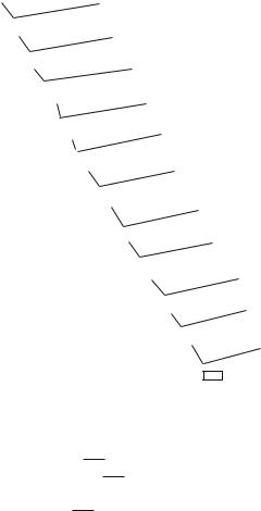
It is convenient to illustrate our application of resolution by means of the tree in Fig. 4.1.
114 |
|
|
|
|
|
|
|
|
|
|
|
4 The Satisfiability Problem and Its Extensions |
|||||||||||||||||||||
X11 X12 |
|
|
|
|
|
|
|
|
|
|
|
|
|
|
|
|
|
|
|
|
|
|
|
|
|
|
|
|
|||||
|
X11 |
X21 |
|
|
|
|
|
|
|
|
|
|
|
|
|
|
|
|
|
|
|
|
|||||||||||
|
|
|
|
|
|
X21 X22 |
|
|
|
|
|
|
|
|
|
|
|
|
|
|
|
|
|
|
|
|
|||||||
X12 X21 |
|
|
|
|
|
|
|
|
|
|
|
|
|
|
|
|
|
|
|
|
|
|
|
||||||||||
X12 X22 |
|
|
|
|
|
|
|
|
|
|
|
|
|
|
|
|
|
|
|
|
|
|
|||||||||||
|
X12 X32 |
|
|
|
|
|
|
|
|||||||||||||||||||||||||
|
|
|
|
|
|
|
|
|
|
|
|
|
|
|
|
|
|
|
|
|
|
|
|
|
|
|
|
|
|
|
|
|
|
|
X22 X32 |
|
|
|
|
X22 |
X32 |
|
|
|
|
|
|
|
|||||||||||||||||||
|
|
|
|
|
|
|
|
|
|
|
X31 X32 |
|
|
|
|
|
|
|
|||||||||||||||
|
|
|
X32 |
|
|
|
|
|
|
|
|
|
|
|
|
|
|||||||||||||||||
|
|
|
|
X31 |
|
|
|
|
|
|
|
|
|
|
|
|
|
|
|
|
|
|
|
|
|
|
|
||||||
|
|
|
|
|
|
|
|
|
|
|
|
|
|
X11 X31 |
|
|
|
|
|
|
|
||||||||||||
|
|
|
|
|
|
|
|
|
|
|
|
|
|
|
|
X11 X12 |
|||||||||||||||||
|
|
|
|
|
|
|
X11 |
|
|
|
|
|
|
||||||||||||||||||||
|
|
|
|
|
|
|
|
|
|
X12 |
|
|
|
|
|
|
|
|
|
|
|
|
|
|
|
|
|
|
|
|
|||
|
|
|
|
|
|
|
|
|
|
|
|
|
|
|
|
|
|
|
X12 |
X22 |
|||||||||||||
|
|
|
|
|
|
|
|
|
|
|
|
|
|
|
X21 X22 |
||||||||||||||||||
|
|
|
|
|
|
|
|
|
|
|
|
|
X32 |
||||||||||||||||||||
|
|
|
|
|
|
|
|
|
|
|
|
|
|
|
|
|
|
|
|
|
|
|
|
|
|
||||||||
|
|
|
|
|
|
|
|
|
|
|
|
|
|
|
|
|
X21 |
|
|
|
|
X21 X31 |
|||||||||||
|
|
|
|
|
|
|
|
|
|
|
|
|
|
|
|
|
|
|
|
X31 |
|
|
|
|
X31 |
||||||||
Fig. 4.1 A resolution tree
At each level we apply resolution. For example at level 1 we resolve clauses (4.47) and (4.50) to obtain X12 X21 which is then resolved with (4.48). Proceeding
in this way we ultimately resolve X31 with X31 to produce the empty clause represented by ‘ ’ showing that the original statement is not satisfiable.
Note that at the end both X31 and X31 are ‘non-input’ clauses, having been derived in the course of the calculation. This is of importance in distinguishing between ‘easy’ and ‘difficult’ problems and is addressed in Sect. 4.6 and in Exercise 4.12.11.
Given that the statement in Example 4.3 is not satisfiable, what is the maximum number of clauses which can simultaneously be made satisfiable? This is an example of the maximum satisfiability problem.
If we represent a general (disjunctive) clause as a constraint among 0–1 variables in the form of (4.35) (indexed as constraint j) we can force its satisfaction by a 0–1 variable y j taking the value 1. In order to do this we write the constraint as (4.56) using the modelling methods discussed in Chapter 3.
r |
r+s |
|
− xi + |
xi − y j −r |
(4.56) |
i=1 |
i=r+1 |
|
4.5 The Maximum Satisfiability Problem |
|
115 |
By employing the objective |
|
|
Maximise |
y j |
(4.57) |
|
j |
|
we maximise the number of clauses which are satisfied. |
|
|
We apply this model to Example 4.3 to give Maximise |
|
|
y1 + y2 + y3 + y4 + y5 + y6 + y7 + y9 + y9 |
(4.58) |
|
subject to |
|
|
x11 + x12 − y1 0 |
(4.59) |
|
x21 + x22 − y2 0 |
(4.60) |
|
x31 + x32 − y3 0 |
(4.61) |
|
x11 + x21 + y4 2 |
(4.62) |
|
x11 + x32 + y5 2 |
(4.63) |
|
x21 + x31 + y6 2 |
(4.64) |
|
x12 + x22 + y7 2 |
(4.65) |
|
x12 + x32 + y8 2 |
(4.66) |
|
x22 + x32 + y9 2 |
(4.67) |
|
xi j {0, 1}
The LP relaxation produces a fractional solution. Proceeding to an optimal IP solution the maximal objective value is 8, showing that the model is not satisfiable. Among the alternative optimal integer solutions is
x11 = x22 = x32 = 1, x12 = x21 = x31 = 0 |
(4.68) |
y1 = y2 = y3 = y4 = y5 = y6 = y7 = y8 = 1, y9 = 0 |
(4.69) |
i.e. we can satisfy at most eight clauses.
(This has the ‘useless’ interpretation that we can put object 1 in box 1 and objects 2 and 3 in box 2 so satisfying the conditions that every object must be put somewhere but breaking one of the conditions that no more than one object can be put in any one box.) As a variant of the maximum satisfiability problem we might weight clauses differently according to their size. For example we might prefer smaller clauses to larger ones. This could easily be accomplished by giving different weights to the variables in the objective.
Although resolution and absorption produce the minimal size implied clauses their complete sum may contain redundancies, i.e. the conjunction of a proper subset