Both these solutions satisfy the constraints of the original IP model.

The first solution results in an objective value of 63 and the second in an objective value of 68 showing solution (4.149) to be optimal.

If we had only produced one of the satisfying solutions (and not checked if there were others) we could have proceeded by dissecting the interval between the corresponding objective value and 80 progressively seeking, or showing the absence of solutions with larger objective values.

The full execution of use of resolution and the DPL procedure in this example is left as Exercise 4.12.24.

An alternative approach to examples such as this would be to use the LP relaxation to obtain upper bounds on the optimal objective value at each stage. These bounds could then be used as the right-hand side on the (objective) constraint. Also IP constraints could then be produced as ‘cutting planes’ from some of the resultant logical clauses in the manner described in Sect. 4.3. The application of this procedure to Example 4.6 is left as Exercise 4.12.26.

4.10 Applications

In this section we describe some practical problems that are particularly suited to being viewed as satisfiability problems, or extensions of this problem. They are often most satisfactorily solved using the methods of IP.

4.10.1 Electrical Circuit Design Using Switches

Suppose we wish to allow electric current to pass through a set of wires only if certain combinations of switches are on. There will be many ways of achieving this. Normally we will seek an ‘economical’ solution. Possible objectives are as follows:

i.Minimising the number of switches.

ii.Minimising the wire length.

iii.Minimising the number of junctions.

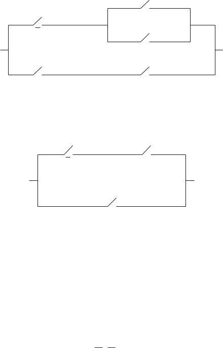
For example, Fig. 4.8 illustrates a circuit, with redundancies, which represents the logical statement (in DNF):

Simplifying (4.150) (by consensus and absorption) we obtain

X1

X2

X3

Fig. 4.8 A redundant electrical circuit

These two prime implicants represent the smallest statement in terms of both the number of clauses and number of literals. The result translates into the circuit in Fig. 4.9.

X1

Fig. 4.9 A simplified electrical circuit

For more complicated circuits we would need to specify the exact objective and use the methods described in Section 4.5.

4.10.2 Logical Net Design Using Gates

Electronic components exist to perform different logic functions. In particular if one has components which perform one of the complete connectives, discussed in Chapter 1, then one can construct any logic function out of them by connecting together a number of these components. For example a common gate used performs the NOR function (the connective arrow ‘↓’). It is shown in Fig. 4.10.

This gate gives a signal Y when, and only when, neither input X1 nor input X2

is present, i.e. the logical function X1 · X2. By connecting together such gates one can perform any logical function. For example the logical statement

(known as ‘exclusive or’) is realised by the net in Fig. 4.11.

The minimum DNF or CNF realisation of (4.152) is of little use in designing a structure with the minimum number of gates to perform the function. Another ‘normal form’ is needed. However, the problem can be formulated as an IP and is set as Exercise 4.12.20. In fact Fig. 4.11 is the minimal representation.

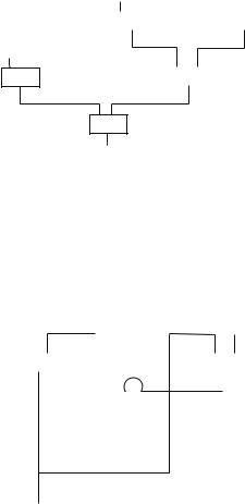
It is worth pointing out that gates, such as NOR, can be connected to each other to give control systems with a ‘memory’. For example Fig. 4.12 represents a ‘flip-flop’.

Fig. 4.12 A flip-flop

If the X1 signal comes before X2 then the first NOR gate is switched off. The only output will be Y2. On the other hand if X2 precedes X1 the only output will be Y1. The logic of optimally designing systems with memory is beyond the scope of this book but can be achieved by IP.

Many other gates are manufactured in practice performing functions such as NAND, XOR (exclusive or), OR, etc.

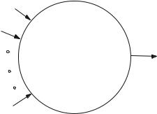
A particularly important class of gates is known as ‘threshold gates’. These have a number of inputs (n) which multiply the 0–1 input signals by given amounts a1,a2, . . . , an and only produce an output if the combined input reaches some designated threshold level b or more. A threshold gate is illustrated in Fig. 4.13.

a1

a2

b

an

Fig. 4.13 A threshold gate

If the inputs are represented by 0–1 variables x1, x2, . . . , xn then the gate produces only an output if the knapsack constraint

is satisfied.

It is possible to create all the logic functions by individual or combinations of threshold functions. Exercise 4.12.22 addresses this question but further discussion is beyond the scope of this book.

All the design problems discussed here are usually considered under the heading of VLSI (very large-scale integrated circuit) design.

4.10.3 The Logical Analysis of Data (LAD)

A major application of computational logic is to finding ‘economical’ (or minimum size) logical formulae which can be used to predict a result from certain input data. Important areas are disease diagnosis, credit scoring, pattern recognition, data compression in order to transmit or store digital data and the design of safety systems. The data are converted into a finite set of true/false observations. If necessary continuous measurements are converted into 0–1 statements, e.g.

We motivate the discussion by a medical example.

Example 4.7 Create a minimal logical formula to diagnose the occurrence of a disease as a result of the following observations:

‘T’ and ‘F’ denote positive and negative symptoms, respectively, and ‘–’ indicates irrelevance of the symptom for the particular test.

In order to obtain a logical formula for predicting the disease we first express the presence of a symptom Si by a literal Xi .

Table 4.2 is represented in DNF as follows:

X1 · X2 · X4 X1 · X2 · X4 · X5 X1 · X2 · X3 · X4 X1 · X3 · X4 (4.155)

Applying consensus and absorption we obtain the complete disjunction of prime implicants as

By means of a truth table or IP we can show that none of the prime implicants is redundant. Therefore (4.156) represents the minimum equivalent statement to Table 4.2 in DNF. However, we also need to ensure that Table 4.3 is consistent with Table 4.2.

Table 4.3 is represented by

Since this statement needs to be false, if the patient has the disease, we negate it using De Morgan’s laws to give (in CNF)