


2.3 The Use of 0–1 Variables |
55 |
into one another. In all these types of models, with some applications, objectives with non-unit coefficients may be used.
2.3.7 Non-linear Problems
Example 2.17 demonstrates how a certain type of non-linearity in an IP model may be linearised. Non-linear models in general may be remodelled, to a degree of approximation and an increase in size, as linear IP models. Hence the distinction between linear and non-linear in IP is less important than in other branches of mathematics. What’s more the IP formulation has the advantage that global optimal solutions are obtained in contrast to local optimal solutions. This distinction is illustrated in Fig. 2.14.
y
global optimum
local optimum
local optimum
Fig. 2.14 Local and global optima
If our objective were to maximise y then conventional optimising methods might find one of the local optima shown and not be able to improve on these. However, an IP formulation can be guaranteed to find a global optimum (at, possibly, considerable computational cost). The next example illustrates how non-linear models may be formulated as linear IP models.
Example 2.17 Make a piecewise linear approximation to the non-linear function y = x3 − 12x2 + 23x + 86 for 0 x 39 and model the (approximate) relationship between x and y using an IP model.
Such an expression (together with other non-linear expressions) may occur in the objective, the constraints or both.
Figure 2.15 gives the graph of y = x3 − 12x2 + 23x + 86.
We evaluate the function at a number of grid points. These need not necessarily be evenly spaced, but for this example we evaluate the function at integers between x = 0 and 9 giving Table 2.1.

56 |
2 Integer Programming |
Y
B
C
A
Q
P D
E J
F
I
G
H
X
Fig. 2.15 A piecewise linear approximation to a non-linear function
|
|
Table 2.1 |
Values for a Non-linear Function |
|
|
|||||
x |
0 |
1 |
2 |
3 |
4 |
5 |
6 |
7 |
8 |
9 |
y |
86 |
98 |
92 |
74 |
50 |
26 |
8 |
2 |
14 |
50 |
|
|
|
|
|
|
|
|
|
|
|
Joining these points in Fig. 2.15 gives the piecewise linear approximation ABCDEFGHIJ to the curve for the function. In order to do this we introduce (non-negative continuous) variables λ0, λ1, λ2, λ3, λ4, λ5, λ6, λ7, λ8, λ9 which represent ‘weights’ given to the points A,B,C,D,E,F,G,H,I,J in representing the function by the following equations:
x = 0λ0 + 1λ1 + 2λ2 + 3λ3 + 4λ4 + 5λ5 + 6λ6 + 7λ7 + 8λ8 + 9λ9 (2.111)
y = 86λ0 + 98λ1 + 92λ2 + 74λ3 + 50λ4 + 26λ5 + 8λ6 + 2λ7 + 14λ8 + 50λ9
|
(2.112) |
λ0 + λ1 + λ2 + λ3 + λ4 + λ5 + λ6 + λ7 + λ8 + λ9 = 1 |
(2.113) |
λ0, λ1, λ2, λ3, λ4, λ5, λ6, λ7, λ8, λ9 0 |
(2.114) |
λ0, λ1, λ2, λ3, λ4, λ5, λ6, λ7, λ8, λ9 R |
|
2.3 The Use of 0–1 Variables |
57 |
In addition we need to impose the condition |
|
At most 2 adjacent λi can be non-zero |
(2.115) |
If λi and λi+1 are the two adjacent non-zero λi ’s then (x, y) represents a point on
the line between the points corresponding to the ith and (i + 1)th grid points. For example if λ0 = 0, λ1 = 0, λ2 = 14 , λ3 = 34 , λ4, . . . , λ9 = 0 then (x, y) = (2 34 , 78 12 ) being the point P in Fig. 2.15. On the true curve if x = 2 34 then y = 79 1964 being
the point Q. The piecewise linear approximation has therefore underestimated the true value of y by 5164 . Obviously the more refined the grid the more accurate the approximation, but more λi variables will be needed.
It remains to represent condition (2.115) by constraints. In order to do this integer variables are needed. We need to model the logical condition that the possible nonzero pair is either λ0 and λ1, or λ1 and λ2, or λ3 and λ4, etc. This can be done by
0–1 variables δ1, δ2, . . . , δ9 and the constraints |
|
|
|
λ0 δ1 |
(2.116) |
λ1 |
δ1 + δ2 |
(2.117) |
λ2 |
δ2 + δ3 |
(2.118) |
|
. |
|
|
. |
|
|
. |
|
λ8 |
δ8 + δ9 |
(2.119) |
|
λ9 δ9 |
(2.120) |
δ1 + δ2 + δ3 + δ4 + δ5 + δ6 + δ7 + δ8 + δ9 = 1 |
(2.121) |
|
Constraint (2.121) ensures that exactly one δi is 1, the others being 0. Then by constraints (2.116)–(2.120) at most two adjacent λi can be non-zero.
In order to ‘linearise’ expressions such as that above in this way they must be functions of a single variable or be able to be expressed as the sum of non-linear functions of single variables. Such functions are known as ‘separable.’ The limitation of only being able to model separable functions is not as restrictive as might, at first, be thought. For most functions arising in practice it is usually possible to ‘separate’ them by suitable transformations. For
example |
the product |
x y |
of |
two continuous |
variables, although not separable, |
can be |
transformed |
into |
a |
separable model |
by the log transformation since |
log x y = log x + log y.
We again discuss how non-linear problems give rise to IP models and the important distinction between convex and non-convex models in Chapter 3.
58 |
2 Integer Programming |
2.3.8 The Knapsack Problem
This is one of the simplest types of pure IP model involving only one constraint and takes the form
Maximise
c j x j |
(2.122) |
|
j |
|
|
subject to |
|
|
a j x j |
b |
(2.123) |
j |
|
|
x j 0 |
j |
(2.124) |
x j Z |
j |
|
Like some of the other IP models discussed in Sect. 2.4, under the title of ‘computational complexity’, this type of model is ‘difficult’ to solve but, in one sense, the easiest of such IP models. Extensions of the knapsack problem are the bounded variable knapsack problem, the 0–1 knapsack problem and the equality-constrained knapsack problem. The name arises from the largely fictitious application of trying to fill a knapsack of limited size with items of maximal total value (although it has been used to allocate the hardware for different experiments in space exploration vehicles). More commonly it is used as a subproblem for other combinatorial problems (e.g. cutting stock and bandwidth allocation).
The LP relaxation of the knapsack problem is trivial to solve (concentrate on the activity with the greatest ratio of objective coefficient/constraint coefficient) but the IP involves finding the best combination of items to fill the knapsack taking account of both this ratio and how well it fits (with other items) into the knapsack.
2.3.9 The Travelling Salesman Problem
We demonstrate this problem by the following example.
Example 2.18 A routing problem. Find the shortest order to go around cities N = {1, 2, . . . , n}, returning to the beginning. The distance from city i → j is given as ci j .
We will assume that the distance from i to j is not, necessarily, the same as the distance from j to i, i.e. we have an example of the asymmetric travelling salesman problem (TSP).
We can model this problem as
2.3 The Use of 0–1 Variables |
|
|
59 |
Minimise |
|
|
|
|
ci j xi j |
(2.125) |
|
i, j |
|
|
|
subject to |
|
|
|
xi j |
= 1 |
i N |
(2.126) |
j |
|
|
|
xi j |
= 1 |
j N |
(2.127) |
i |
|
|
|
xi j |S| − 1 S N such that 1 < |S| < n |
(2.128) |
||
i, j S |
|
|
|
xi j {0, 1} i, j N
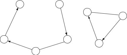
The 0–1 variables xi j indicate whether a direct link i → j is, or is not, on the tour. Constraint (2.126) forces each city to be left exactly once and constraint (2.127) forces each city to be entered exactly once. Constraint (2.128) rules out subtours. Figure 2.16 demonstrates subtours which would be ruled out by constraints (2.128). Note that there are 2n − n − 1 subtour elimination constraints, i.e. an exponential number as a function of n. In practice these constraints are only added on an ‘as needed basis’, or known facet constraints are added when they cut off fractional solutions to the LP relaxation.
1  6
6
3
 7
7
4 |
8 |
5
2 
Fig. 2.16 Subtours of a TSP
There are other formulations of the TSP, as an IP, with a polynomial number of constraints although they have weaker LP relaxations (with one exception). References are given in Sect. 2.5.