of the prime implications may be equivalent to the original statement. We illustrate this by an example.

4.6 Simplest Equivalent Logical Statement

Example 4.4 What is the minimum number of prime (disjunctive) clauses whose conjunction is equivalent to the following statement?

Applying resolution and absorption successively delivers the following set of prime implications, giving the following equivalent statement:

There may be a proper subset of these prime implications, the conjunction of which is also equivalent to the original statement. We give an IP formulation later. We can solve this example by means of a truth table with 32 rows. It is sufficient to find a subset of the clauses the truth of which implies the truth of all the clauses. (Implication the other way follows from the fact that the clauses are already prime implications.) Therefore we need to find a subset, the truth of which implies the truth of the other clauses.

It can be shown that the first five clauses imply the sixth. Also the first four and the sixth clause imply the fifth. No smaller subset implies the others. Therefore there are two shortest equivalent statements. They are

In practice heuristics are often used to find, hopefully good, but suboptimal solutions to this problem. However, in this book, we concentrate on exact methods.

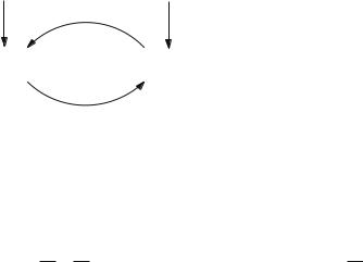
Figure 4.2 demonstrates the dependencies of the prime implications.

Fig. 4.2 Dependency between prime implications

If a clause has arrows leading into it then it is the result of successive resolutions applied to the clauses from where the arrows originate and the resultant clauses. It is therefore redundant when all the clauses at the origins of the arrows are present.

of X1 X2 X3 and X1 X4. Therefore X1 X2 X3 and X2 X3 X4 are each only redundant if the other is present.

We can use the dependency diagram to give an IP formulation of the problem of finding the minimum sum of prime implications. We introduce 0–1 variables yi which are 1 if the corresponding clause is present. For each clause we keep track of which sets (if any) of prime implication clauses give rise to it by successive resolutions applied to them. Then this clause is redundant if any of the origin sets of clauses is present. Each origin set of clauses {i1, i2, . . . , ir } is represented by a 0–1 variable zi1,i2,...,ir which takes the value 1 if all the clauses in the set are present.

Clause i may have a number of alternative origin sets Si1, Si2, . . . , SiM . In order to avoid ignoring any origin set we must suspend the absorption operation when using resolution for this purpose. Clause i can only be removed if all the clauses in one of the origin sets is present. Therefore we stipulate

118 4 The Satisfiability Problem and Its Extensions

We can simplify a statement in DNF to produce its prime implicants using the (logical) dual of resolution. A prime implicant is a conjunctive clause which implies the original statement and is such that no smaller clause containing a subset of the literals with the same sign implies the statement. The corresponding operation to resolution is known as consensus. A consensus of two (conjunctive) clauses with overlapping literals of the same sign, except for one literal, is obtained by taking their conjunction and deleting the common literal which is negated in one and unnegated in the other. For example the consensus of

The consensus clearly implies the pair of clauses from which it is derived. It is added to the set of clauses.

We also apply absorption. If one conjunctive clause contains literals (of the same sign) which are a subset of the other then the larger clause is redundant and is removed. If we successively apply consensus and absorption to a statement in DNF we obtain the disjunction of all the prime implicants. This statement is equivalent to the original statement. Note the distinction between simplification in DNF and CNF. In CNF we obtain prime implications but in DNF we obtain prime implicants. But analogous to the CNF case, the disjunction of a proper subset of these prime

implicants may also be equivalent to the original statement. In order to illustrate this let us consider the negation of the statement in Example 4.4. Using De Morgan’s laws (as described in Chapter 1) this is naturally written in DNF by interchanging ‘·’ and ‘ ’ and changing the sign of each literal. Applying consensus and absorption delivers us the logical dual of (3.80)–(3.85), i.e.

(X1 · X4) (X1 · X4) (X2 · X5) (X3 · X5) (X1 · X2 · X3) (X2 · X3 · X4) (4.101)

The minimum disjunction of prime implicants, giving an equivalent statement, consists of either the first five or the first four and the sixth of the above conjunctive clauses corresponding to the duals of (3.86) and (3.87).

We have confined our attention to minimising the number of clauses in an equivalent statement (whether in CNF or DNF). Alternatively we might wish to minimise the total number of literals in the equivalent statement. In order to do this we would weight clauses according to their size in the minimisation. For the example this still results in (4.86) and (4.87).

It will clearly never be the case that the statement using the minimum number of literals does not use prime implications (or prime implicants in the DNF case).

CNF and DNF are only two of the normal forms which we might wish to minimise. As discussed in Chapter 1 there are many ways to represent a logical statement as well as different connectives which can be used. In practical terms the relevant form to use depends on the problem being considered. For example in Sect. 4.10 we discuss different forms of logical circuit design where we might wish to minimise the number of switches or gates, or some other aspects of the architecture.

4.7 Horn Clauses: Simple Satisfiability Problems

The satisfiability problem and its extensions are very difficult problems to solve in the worst case (they are NP hard) whether they are solved by logical or IP methods.

However there are special cases that are comparatively easy to solve. One such is when all the clauses are Horn clauses. These are statements which can be written in the form

or

i.e. they can be written as implications where the premises are conjunctions of unnegated literals and the consequents are either single unnegated literals or tautologies (always true). Written as disjunctive clauses (4.102) and (4.103) are

Hence Horn clauses, expressed as disjunctions, contain at most one unnegated literal. This makes such systems particularly easy to solve (the number of steps is always a polynomial function – which can be made a linear function – of the size of the problem). A number of logic programming systems restrict themselves to rules of this form for this reason. Some systems that are not Horn can be made such by a simple transformation of variables (e.g. replacing unnegated literals by negated ones, throughout the system, or vice versa). Such systems are called essentially Horn.

We illustrate the situation by means of the following example.

Example 4.5 From the following set of Horn clauses is it valid to deduce X2 ?

As explained, at the beginning of this chapter, we negate the conclusion, appending

as an extra Horn clause and test the satisfiability of the system. If it is not satisfiable then the conclusion X2 is valid. (Alternatively we could deduce all the prime

implications of the original system to see if X2 is one of them.)

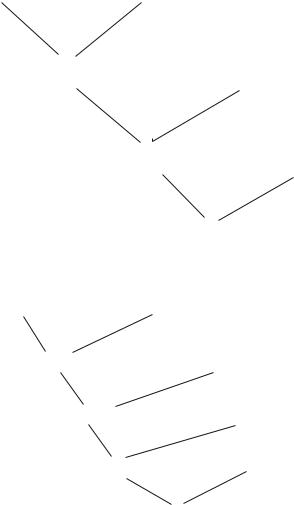
If we apply resolution to the system we obtain the tree in Fig. 4.3.

Notice that one of the two clauses in each resolution operation is one of the input clauses. This is in contrast to Fig. 4.1 where the last resolution was between two non-input clauses. If each resolution involves an input clause it is only necessary to store them and the current resolved clause. This leads to a reduction in the amount of computation to a polynomial number of steps. (In fact it can be made a linear number of steps.) In order to see why input resolution is sufficient for delivering all the prime implications of a Horn clause system we consider the following (totally general) example of two successive resolutions illustrated in Fig. 4.4.

C1, C2, C3, C4 are disjunctive clauses and the input clauses are at the top level. In order for the system to be Horn and for the resolutions to be possible we stipulate

C1 C2 C3 C4

Fig. 4.4 Non-input resolution in a Horn system

that all the literals in C1, C2, C3 and C4 are negated. (Some literals may be shared in common.)

At the top level we eliminate X1 and X2, respectively, and at the next level we eliminate X3.

Observe that Fig. 4.4 illustrates a non-input resolution since both clauses at the second level are non-input. But it is possible to derive the same result by the input resolution illustrated in Fig. 4.5.

Therefore we can restrict ourselves to input resolution when we have Horn systems. Another feature of Horn systems, worth remarking on, is that they are closed under resolution. Each resolved clause is itself Horn.

It also turns out that the corresponding IP model for a Horn system is particularly easy to solve. We illustrate the combining of constraints in such a model, corresponding to Example 4.5, in Fig. 4.6.

In order to simplify the presentation we do not explicitly include the constraints xi 0 and −xi −1 which are added, where necessary, to make coefficients equal.

C1 C2 C3 C4

Fig. 4.5 Input resolution in a Horn system

−8x2 >= − 7

Fig. 4.6 Input resolution for an equation system

The final constraint, after rounding, clearly demonstrates that x2 = 0.

Figure 4.6 also shows that, with input resolution applied to constraints, we can postpone rounding until the end. Consider a constraint representing a Horn clause.

i=1